Download
1 / 21
260 likes | 509 Views
MOTION, MOTION, MOTION... The motions of macroscopic bodies (bullets, baseballs, and planets) are perfectly described by the laws of Newton. In classical mechanics we deal with what are called dynamical variables . These are position, momentum (linear and angular), and energy.

E N D
MOTION, MOTION, MOTION... The motions of macroscopic bodies (bullets, baseballs, and planets) are perfectly described by the laws of Newton. In classical mechanics we deal with what are called dynamical variables. These are position, momentum (linear and angular), and energy. A dynamical variable that can be measured is called an observable. The state of a macroscopic body at any time is specified completely by the position coordinates (x, y, and z) and the coordinates of the momenta (px, py, and pz) at the time in question. Since momentum is the product of mass with velocity we could use the velocity coordinates (vx, vy, and vz) instead of the momenta. The three-dimensional path that is taken by a body in motion as a function of time is called its trajectory. This trajectory is the full description of the motion of the particle throughout its coordinate system.
Newton's Second Law enables us to calculate the trajectory of a particle in terms of the forces acting on it. Thus the entire history and the entire future of the body's motion, point by point, can be computed from the knowledge of the current position of the particle and the magnitude and direction of the forces acting upon it. Newton's laws are in this sense deterministic. This is the property that enables our Astronomy colleagues to compute the trajectory of the planets and to accurately predict the occurrence of future phenomena such as solstices and eclipses.
Newton’s Second Law is a Law of Motion and is usually formulated as where a (or ) is the acceleration imparted on the mass m under the application of the force F. The Uncertainty Principle (to be discussed later) is of no practical importance for the motions of macroscopic bodies. Because we can determine both their position and momentum simultaneously with arbitrary precision. However, as we shall see, this is not the case when we wish to compute the motions in the sub-microscopic world of atoms, molecules, nuclei, and electrons. See Module 1 for some discussion on the Bohr model of the H atom.
The laws that govern our everyday human world such as Newton's laws of motion and the laws of Thermodynamics are postulates. This means that they cannot be derived from other, more fundamental laws. Postulates cannot be proven, but if other rules or properties that are derived from postulates are shown by experiment to be true, then we can say that the postulates are consistent with our experience (e.g., the laws of Thermodynamics) The laws of quantum mechanics can also be posed in the form of postulates. The difference being that the postulates that govern our everyday world are apparent and sensible to us; those that govern the micro-world are much more abstract. Some postulates of quantum mechanics are now presented here.
POSTULATE 1 "The state of a system of particles is completely specified by a function (Y) )that depends on the coordinates of the various particles, and on time. All possible information about the system can be derived from this function." POSTULATE 1A “The probability that a particle will be found at a specific time t, in a volume element dt at the point r is proportional to POSTULATE 2 "For every observable (dynamical variable that is experimentally measurable) there exists a linear, Hermitian operator." POSTULATE 3 “The wavefunction Y(r1, r2, …, t) changes in time according to Where Ĥ is the hamiltonian operator
POSTULATE 1 "The state of a system of particles is completely specified by a function that depends on the coordinates of the various particles, and on time. All possible information about the system can be derived from this function." this function is commonly termed the wavefunction, or state function. the phrase "all possible information" refers to the information about the system that is open to experimental determination (the observables). the wave function is usually represented by Y(r1, r2,…, t), where r1, r2,… are the spatial coordinates (with respect to some origin) of particles 1, 2, …, that make up the system, and t is the time. the spatial and temporal components of Ycan be separated. By convention we denote the time-independent wavefunction by y (lower case, italic). Often chemists are concerned only with the spatial characteristics of a system (the shape of a compound) and are unconcerned with how it changes with time. Not so for Photoscientists!!!
Y is a mathematical function that carries all the information. What we need to do is to find some means to unlock the information from Y. Much in the same way that we can unlock information about real compounds, such as benzene, by carrying out some appropriate experiments. We must find some way to work on Yto cause it to give us the same information that we could obtain through experiments. Later we shall see how to do this.
A chemical system can exist in many stationary states. The symbol y (time-independent) denotes a math function that carries information on all stationary states of the system. But we may want more specific information, e.g. the energy of a particular stationary state (position variables only) of a molecule or atom. In such cases wavefunctions are qualified by quantum numbers that can specify the appropriate wave function for particular variables. Such wavefunctions may appear as ym,n,… where m, n, etc are quantum numbers that represent the particular subsets of y that interest us. We can also refer to the particular state of a system using its quantum numbers only, with y implied. E.g. the wavefunction ya, b, c can be simply denoted by [a,b,c]. In the Dirac bra-ket system ymand ym* (the complex conjugate of ym) are represented by , respectively.
Acceptable Wavefunctions • Wavefunctions are mathematical entities that denote real systems and therefore they must make some kind of physical sense. • Because of this there are certain limitations that need to be placed on the wavefunctions. • Such wavefunctions are said to be well behaved. • The criteria for this (using only the x dimension) are: • At any x, y(x) must have only one value (single-valued). • y(x) and dy(x)/dx must be continuous. • (iii)y(x) must not be infinite over a finite range (but it can be infinite over an infinitesimally small range). • y(x) must be square integrable, i.e. • must be a finite quantity.
About complex conjugates: Note that if y = a + ib, then y* = a – ib and yy* = (a + ib)(a - ib) = a2 + b2 and yy* is thus real and non-negative
The square integrable condition requires that the definite integral shown above must not be equal to zero or to infinity, it must be a finite quantity. (we shall return to this point shortly) POSTULATE 1A This concerns the interpretation of the wavefunction itself. The probability that a particle will be found at a specific time t, in a volume element dt at the point r is proportional to In one-dimensional motion the product represents the probability of finding the particle between x and x + dx, at the time t.
In a 3-dimensional situation, the postulate tells us that the probability of finding the particle in some small volume element is given by Pr = Y2dt (or Pr = Y*Y dt if Y is complex) the quantity Y2 can be thought of as a probability densityin the sense that it generates a probability when it is multiplied by the volume element, dt. The wavefunction itself is a probability amplitude and has no physical meaning, per se. This interpretation is due to Max Born (1926) He argued that probability is measurable (at least in principle) and as such it must be a real, non-negative quantity, and it therefore must relate to a real, non-negative quantity arising out of the wavefunction. Wavefunctions must be well behaved but they can be real or complex, positive or negative. Born postulated that the correct identity was given by the product of the wavefunction with itself, or with its complex conjugate when the function contains imaginary quantities.
The Born postulate highlights the difference between classical and quantum mechanics. In classical terms we can precisely locate a particle as having unit probability of being at a particular narrow range of x-values (between x and dx). Everywhere else on the x-dimension the probability is zero. In quantum terms we equate the measured probability of finding the particle at any value of x to Y2 or the product of Y*Y. Since the wavefunction can have non-zero values for finite values of x, we find ourselves unable to locate the particle at a definite point on the axis. All we can do is to predict the probability of finding the particle at a given value of x, if we know Y(x,t) . The nature of quantum science is that it is statistical, not deterministic. Note, however that particles are not behaving like waves, but it is their probability patterns that satisfy a wavefunction.
One important implication of the Born postulate is that (the square integrable condition). there must be a finite probability of finding the particle somewhere within the region "all space". If, in a given case, the integral above equals a real constant N, then dividing y(x) by N1/2 results in the integral having the value 1.0, i.e. Now the wave function is said to be normalized and the probability is unity for finding the particle in "all space“, as it must be.
POSTULATE 2 "For every observable (dynamical variable that is experimentally measurable) there exists a linear, Hermitian operator." An operator is a symbolic form that tells us to perform a mathematical transposition (operation) on the function that follows the symbol. Thus are all operators that tell us to take the square root, take the derivative with respect to x, multiply by x, and take the sine of, respectively, whatever follows the operator symbol. Barrante, chapter 10 and Math Module B on the our web site develop operator algebra and define linear and Hermitian operators. operators are usually written with a caret “^” over the symbol.
EXPERIMENT SYSTEM OBSERVABLE WAVEFUNCTION OPERATOR Thus it is the application of the appropriate operator that unlocks the related observable from the wavefunction. We can bring postulates 1 and 2 together as a diagram The postulates examined to date enable us to calculate observables for a few simple systems. But there is a practical consideration of constructing operators for the observables we wish to calculate.
Constructing Quantum Mechanical Operators for Observables write down the classical expression for the observable we are concerned with in terms of the classical position coordinates and momentum. Replace the position-dependent quantities by the appropriate form of the multiplication operator. Replace the momentum quantities by where q is the position variable. (Do not try to understand this. It can be demonstrated that it is legitimate by employing a mathematical device called a Poisson bracket. We need to simply accept this transform). Other variables (e.g. time, dielectric constant) retain their classical form
For example let us find the operator for energy Newton’s equations of motion are convenient to use if the problem to be solved is cast in the form of Cartesian coordinates, but in other coordinate systems (e.g. spherical) Newton’s equations become cumbersome. In the 19th century Joseph Lagrange and William Rowan Hamilton independently developed equations of motion that were independent of the coordinate system. The approach of Hamilton is the one that best allows the transformation from classical to quantum mechanics. In conservative systems (in which the total energy remains constant with time) the Hamilton function is equal to the total energy of the system expressed in terms of the coordinates of the particles and their conjugate momenta. In a Cartesian system these are x,y, and z, and px, py, and pz.
Assume that we are interested in a single particle only that is constrained to move on the x-axis then the Hamilton function (H) is the sum of the kinetic (T) and potential (V) energies of the particle and Total energy if m = mass and v = velocity, then And in terms of momentum The potential energy (V) depends only on the position on x and thus the Hamilton function is given by
Now we have an expression for total energy (kinetic and potential) in terms of position and momentum using our rules for the construction of operators we form a Hamiltonian operator. In the x dimension, the operator for kinetic energy is thus In 3 dimensions this becomes Where (del) is the Laplacian operator
The potential energy of a particle in one dimension is a function of its position with respect to some origin/baseline. Thus V(x), becomes multiplication by the operator The same is true for 2 or 3 dimensions. Thus the Hamiltonian operator for a particle of mass m, with motion restricted to the x dimension can be written as