Download
1 / 18
190 likes | 316 Views
Remotely sensed land cover heterogeneity. Mao- Ning Tuanmu 5/29/2012. Outline. Objectives & rationale Remotely sensed data Heterogeneity metrics Calculation approaches of heterogeneity metrics Next steps. Spatial heterogeneity of land cover.

E N D
Remotely sensed land cover heterogeneity Mao-NingTuanmu 5/29/2012
Outline • Objectives & rationale • Remotely sensed data • Heterogeneity metrics • Calculation approaches of heterogeneity metrics • Next steps
Spatial heterogeneity of land cover • Species distributions and biodiversity patterns • Landscape metrics based on categorical land cover maps • Boundary delineation • Heterogeneity within a land cover type • Continuous measures of land surface characteristics from remote sensing
Objectives • To explore different approaches for quantifying land cover heterogeneity based on remotely sensed data • To generate remote sensing-based heterogeneity metrics at the global scale • To evaluate the usefulness of those metrics for explaining biodiversity patterns and monitoring their temporal dynamics
Remote Sensing Imagery • Landsat 5 TM and Landsat 7 ETM+ • Global Land Survey (GLS) surface reflectance • 7 bands, QA • Three epochs: 1990, 2000, 2005 • 7,000~8,000+ scenes for each epoch • 22 scenes covering the entire Oregon • Vegetation indices • NDVI
Remote Sensing-Based Metrics • First-order texture measures • Statistics calculated from image pixel values • Composition of pixel values • Average, SD, range, maximum, minimum and etc. of pixel values within a pixel neighborhood • Valuesof individual spectral bands • Linear or non-linear combinations of spectral bands
First-order Texture Measures Standard deviation Coefficient of variation
Remote Sensing-Based Metrics • Second-order texture measures • Statistics calculated based on values of pixel pairs • Information on the spatial relationship between two pixels • Spatial configuration (or arrangement) of pixel values • Metrics based on the Gray Level Co-occurrence Matrix (GLCM)
Gray Level Co-occurrence Matrix (GLCM) • A tabulation of how often different combinations of pixel brightness values (grey levels) occur in a pixel neighborhood • A symmetric n-by-n matrix, where n is the number of all possible gray levels (e.g., n=16 (2^4) for a 4-bit image) • The element Pij of a GLCM is the occurrence probability of the pixel pairs with values i and j within a pixel neighborhood
GLCM Metrics • Pixel neighborhood • Pixel pairs • Direction (0°, 90°, 45°, 135°) • Offset distance (offset = 0) • Metrics • Contrast-related • Contrast, dissimilarity, homogeneity • Orderliness-related • Angular second moment, entropy • Descriptive statistics • Mean, variance, correlation
Second-order Texture Measures Angular second moment Homogeneity
Second-order Texture Measures Contrast Correlation
Moving Window vs. Fixed Grid • Moving window approach • Run a moving window across the entire image (study area) to calculate first- and second-order metrics for each pixel (e.g., Landsat pixel of 30m) • Aggregate metric values (e.g., calculate mean and SD) for a larger regular grid (e.g., MODIS 500m grid) or specific area (e.g., sampling plot) • Fixed grid approach • Directly calculate metrics based on the values of Landsat pixels within each MODIS pixel
Approach Comparison Homogeneity Angular second moment Moving window approach (Mean of metric values in 3x3 windows) Fixed grid approach (Metric values in MODIS 500m grids)
Approach Comparison Standard Deviation 3x3 moving window 11x11 moving window Moving window approach (Mean of metric values in moving windows) Fixed grid approach (Metric values in MODIS 500m grids)
Moving Window vs. Fixed Grid • Moving window approach • Texture characteristics at different grains (3x3, 11x11…) • Computation-intensive • Fixed grid approach • Texture characteristics at the scale of the fixed grid • Easier to interpret • Much less computation-intensive (> 10 times faster)
Next Steps • Comparison between texture measures and landscape metrics from categorical land cover data (NLCD) • Fragstats • Only in the Windows system • Cannot handle the entire Landsat scene with the moving window approach
Next Steps • Metrics related to spatial autocorrelation • Measures of spatial autocorrelation (e.g., Moran’s I) • Characteristics of variogram (e.g., sill and range) • Seasonality effects • Cropland • Mosaicked images from NASA