Download
1 / 26
260 likes | 403 Views
Multiple Window for Image Contrast Enhancement. By Solomon Jones. OVERVIEW. INTRODUCTION LINEAR BINNING NON-LINEAR BINNING K-MEANS CLUSTERING CLIPPED NON-LINEAR BINNING HISTOGRAM EQUALIZATION INFORMATION GAIN. INTRODUCTION.

E N D
Multiple Window for Image Contrast Enhancement By Solomon Jones
OVERVIEW • INTRODUCTION • LINEAR BINNING • NON-LINEAR BINNING • K-MEANS CLUSTERING • CLIPPED NON-LINEAR BINNING • HISTOGRAM EQUALIZATION • INFORMATION GAIN
INTRODUCTION The medical image processing field has a critical need to enhance medical images (e.g. CT Scans, X-Rays, MRIs, etc.). Contrast enhancement takes the gray level intensities of a particular image and attempts to proportionally redistribute the intensities. Our efforts were directed towards creating contrast over user specific intervals and ranges, thus constructing the concept and term Multiple Window.
INTRODUCTION The general idea behind contrast enhancement, in reference to the medical image processing field, is to improve the visual quality of an image.
INTRODUCTION Generally, an image has the potential of displaying colors that span the entire color spectrum. However, medical images are typically shown in black and white. Black and white images can be theoretically reduced to a collection of gray level intensities; the lightest gray level intensity being white and the darkest gray level intensity being black.
BINNING TECHNIQUES • LINEAR BINNING • CLIPPED LINEAR BINNING • NON-LINEAR BINNING • K-MEANS CLUSTERING • CLIPPED NON-LINEAR BINNING For all techniques, we mapped 12-bit (0-4095) gray level intensities into 8-bit (0-255) gray level intensities for general display purposes
LINEAR BINNING • Linear Binning • In general, linear binning is a technique that can best be • described as a re-mapping of color intensities to a separate range of color intensities, which are in direct proportion or ratio with their original intensities. Furthermore, we can breakdown the term linear binning. The first fraction, linear, implies a straight line, hence the redistribution in direct proportion; the second half, binning, stems from the idea of how many sections (bins) the original image intensities will be re-mapped to.
INFORMATION GAIN • INFORMATION GAIN • The information gain is calculated by subtracting the entropy from the information. Entropy is a measure of the average information content associated with a random outcome and is defined as Σ –P(i)log2 (P(i)); information is defined as a measure of the decrease of uncertainty and is defined as Σ –log2 (P(i)), where P(i) is the probability of selecting a particular gray level. • INFORMATION GAIN = Information – Entropy • INFORMATION = Σ –log2 (P(i)) • ENTROPY = Σ –P(i)log2 (P(i))
INFORMATION GAIN • INFORMATION GAIN RESULTS • Original Image Information Gain = 1038 • LINEAR
CLIPPED LINEAR BINNING • Clipped Linear Binning • The medical image processing field has determined that the majority of soft tissues fall within the inclusive range of 856 and 1368. • When applying this technique, we are only concerned with gray level intensities within the aforementioned range. Any intensity levels strictly below the 856 minimum were reduced to 0 and any intensity levels strictly above 1368 were reduced to 255. • It is important to remember that we were mapping 12-bit values to • 8-bit values, so, we were technically reducing the latter values to 255;
CLIPPED LINEAR BINNING • Clipped Linear Binning (cont.) • The final step in clipped linear binning was to apply a linear bin on the interval or range of values of which inclusively fall between 856 and 1368.
NON-LINEAR BINNING • Non-Linear Binning • Non-linear binning is a considerably more expensive algorithm. The non-linear binning technique first calls for the creation of a histogram matrix, with each row of the matrix numbered from 0 to 4095. • Each cross-section of the matrix (row intensity w/ its corresponding 1 column) held the frequency of that row intensity. • The next step required that we then create random clusters points (centroids) within the range value of the original image.
NON-LINEAR BINNING • Non-Linear Binning (cont.) • We accomplished establishing arbitrary centroids by simply taking • the user’s bin input and dividing the original image range values into equal parts and marking each division as a centroid data point. The first and last centroidswere displaced by only a half interval; all other centroids were displaced a full interval from their preceding centroid. These centroids started out as our initial cluster points. • The K-Means Clustering technique is then applied to the histogram matrix, and once the clustering technique has recalculated its new cluster points, we can then apply a linear mapping of the original image intensities to these new cluster points
K-MEANS CLUSTERING • K-MEANS CLUSTERING • The K-Means Clustering algorithm is essentially the crux of non-linear binning. This particular algorithm is a numerical statistical technique used to determine the number of groups (clusters) in a data set. It attempts to group values based on their distance or approximation to initially random data points (centroids) within the data set. After the first round of this procedure has been completed, the algorithm recalculates the random centroidsby calculating the average of the image intensities it initially grouped. This • process will repeat itself until the initially random data points do not change significantly. That particular process usually takes 3-6 rounds. Our implementation implements 5 rounds of the K-Means Clustering technique.
K-MEANS CLUSTERING Now the centroids are moved to the center of their respective clusters. Steps 2 & 3 are repeated until a suitable level of convergence has been reached. Points are associated with the nearest centroid. Shows the initial randomized centroids and a number of points.
K-MEANS CLUSTERING • K-MEANS CLUSTERING (cont.) • Once we have these values as input, we create two loops. The outer-loop is a loop going from 0 to the bin and the inner-loop is a loop going from the min to the max. Inside the inner-loop we check to see which two centroids each intensity is between. • We then determined which centroid the intensity is closest in distance to. Once we have determined which centroid it is closest to, we then multiply its frequency by its image value and add that product to a cumulative sum.
K-MEANS CLUSTERING • K-MEANS CLUSTERING (cont.) • After applying this method to all image intensities, we take our total sum for each centroid and divide the sum by the total number of frequencies that fall under that particular centroid to calculate each new centroid. We do this procedure for all image intensities, and then return to the non-linear function once the algorithm has gone through and recalculated all cluster values.
INFORMATION GAIN • INFORMATION GAIN RESULTS • Original Image Information Gain = 1038 • NON-LINEAR
HISTOGRAM EQUALIZATION • HISTOGRAM EQUALIZATION • Histogram equalization is a relatively painless algorithm to implement and is • widely used in several image applications because of its simplistic procedure and its convincing effectiveness. • This particular technique allows for areas of lower contrast to gain higher contrast by spreading out the most frequent intensity values, and essentially flattening out the histogram. • The disadvantage is that noise and distortion may be emphasized when using this technique.
HISTOGRAM EQUALIZATION • HISTOGRAM EQUALIZATION (cont.) • We began implementing histogram equalization by creating a histogram matrix, indexed by values ranging from 0 to 4095, similarly to how we began the non-linear binning technique. We then created a cumulative frequency matrix for storing the intensities’ frequencies.
HISTOGRAM EQUALIZATION • HISTOGRAM EQUALIZATION (cont.) Corresponding histogram (red) and cumulative histogram (black) Corresponding histogram (red) and cumulative histogram (black)
HISTOGRAM EQUALIZATION • HISTOGRAM EQUALIZATION (cont.) The same image after histogram equalization An unequalized image
HISTOGRAM EQUALIZATION • HISTOGRAM EQUALIZATION (cont.)
INFORMATION GAIN • INFORMATION GAIN RESULTS • Original Image Information Gain = 1038 • EQUALIZATION