Download
1 / 32
380 likes | 679 Views
Human Visual System. 4c8 Handout 2. Image and Video Compression. We have already seen the need for compression We can use what we have learned in information theory to exploit spatial and temporal redundancy but it is not enough

E N D
Human Visual System 4c8 Handout 2
Image and Video Compression • We have already seen the need for compression • We can use what we have learned in information theory to exploit spatial and temporal redundancy but it is not enough • We must determine ways in which we can exploit redundancy in the way we perceive images. • To do so it is important to understand some relevant aspects of the HVS.
Vision : The Human Visual System (HVS) • Light is focused onto the retina • Retina consist of two types of cell • cones – sensitive to colour and luminance, located near the centre of the retina • rods – located near the periphery of the retina, much more sensitive to light, luminance only, more sensitive to motion, less resolution Lens Pupil Retina Optic Nerve Blind Spot
Vision : The Human Visual System (HVS) • Electrical Impulses from the retina are chanelled by the optic nerve to the Visual Cortex • The Visual Cortex does a whole bunch of smart things including filtering, object recognition, edge detection. Lens Pupil Retina Optic Nerve Blind Spot
Intensity Sensitivity of HVS • Given a background Intensity I, the user is asked to increase the intensity of the circle until it is barely visible. • This experiment demonstrates a phenomenon known as Weber’s Law just noticeable difference in intensity a constant defining a quantum for perceived intensity intensity is the power of the incident visible light
Intensity Sensitivity of HVS • We can express this as a differential equation The solution is • p defines a perceptual intensity scale. Our perception of intensity is linear wrt p. When we talk about intensity values in images we are referring to this scale. • 256 levels are sufficient and hence 8-bits numbers are commonly used to define intensity ranges in images.
Colour Sensitivity • Cone Cells in the eyes convert wavelengths of life into 3 values known as a tri-stimulus • The tri stimulus values encode the relative strengths of each of the 3 colour basis. • Different colours correspond to different mixtures of tri-stimulus values.
The RGB Colour Space • attempts to mimic HVS • requires the definition of 3 colour primaries • CIE RGB red = 700 nm, green = 546.1 nm, blue = 435.8 nm • must determine tristimulus (ie. RGB) values for a mono-chromatic light source as a function of its wavelength. (perceptual studies) These functions are known as colour matching functions and can be used to estimate RGB for any combination of colours. Weber’s Law also applies
YUV and related colour spaces • By convention colour spaces for TV broadcast use a tristimulus of 1 luminance (Y) and 2 chrominance values (U and V) to represent colour. • YUV was used so that Colour TV signals would be backwards compatible on Black and White TV sets. • the luminance of a pel (Y) in the YUV space is approximately Note: exact values of weights vary • the higher weight for green reflects the increased sensitivity of the HVS to luminance in wavelengths corresponding to the colour green.
YUV contd. • U and V values are defined below for PAL • Hence conversion between RGB and YUV is linear =C, where • RGB values can be found from YUV values by calculating the matrix inverse of C.
Examples of Conversions • Black (rgb = [0 0 0]) has yuv = [0 0 0] • White (rgb = [255 255 255]) has yuv = [255 0 0] • Shade of Gray (rgb = [x x x]) has yuv = [x 0 0] • Red (rgb = 255 0 0) has yuv = [76.5 -38.3 111.6] • Green (rgb = [0 255 0]) has yuv = [153 -76.5 -95.6] Note: It is common to scale the U and V components so that it fits inside the range 0 to 255 (add 128 to both values)
YUV Colour Spaces • There are many variations on the YUV colour space • YUV – used in PAL colour TV • YIQ – used in NTSC colour TV • YDbDr – used in SECAM colour TV • YCbCr/YPbPr – used for digital TV and still image / video compression • Conversion from RGB to each of these colour spaces is linear but the conversion coefficients can vary slightly.
RGB v YUV RGB YUV
HSV Colour Space • Often used in for image analysis • H – hue = the shade of a colour (red, green, purple etc.) • S – saturation = colour depth (from “washed out”/grey to vivid) • V – Value = brightness of the colour
HSV Colour Space • Conversion from RGB is non-linear
RGB v HSV RGB Hue Saturation Value HSV
Colour Spaces for Compression • JPEG/MPEG etc. use the YUV (YCbCr) colour space because spatial frequency sensitivity of the HVS can be exploited Spatial frequency is measured in cycles per degree. It can be measured at any orientation. Spatial Frequency N cycles θ
Spatial Frequency Sensitivity (Horizontal) Grating increases in freq. Left to Right Intensity decreases vertically. Sensitivity is given by the perceived height of the columns.
Spatial Frequency Sensitivity • HVS less sensitive to chrominance than luminance • chrominance frequencies > 10 cycles/degree are not perceived • nominal max for luminance is 100 cycles per degree • Max sensitivity is at about 5 degrees/cycle • Vertical Frequency Sensitivity is similar but HVS is less sensitive to lower frequencies
Spatial Freq. ResponseMach Banding Bands appear to be brighter on the left than on the right. This is due to spatial filtering in the visual cortex. This phenomenon is simulated with simple filtering of an image row using a low pass filter with a symmetric impulse response.
Consequences of Colour Sensitivity Original Image 512 x 512 x 3 = 0.64 MB
Subsampling Colour Planes Keep Discard 2:1 in both directions Downsample the U and V chrominance channels and leave the Y channel alone
Downsample the U and V chrominance channels and leave the Y channel alone 4:1 Colour Downsampling OK 512 x 512 + 256 x 256 x 2 = 0.31 MB (1/2 bandwidth of original)
Downsample the U and V chrominance channels and leave the Y channel alone 16:1 Colour Downsampling Still OK 512 x 512 + 128 x 128 x 2 = 0.24 MB (1/3 bandwidth of original)
Downsample all 3 channels evenly 16:1 Luminance Downsampling Not good 128 x 128 x 3 = 0.04 MB (1/16 bandwidth of original) Latex
Chrominance Downsampling • You will often see ratios in the description of codecs • 4:2:0 – means 4:1 Chrominance downsampling (2:1 along rows and columns) • 4:2:2 – 2:1 Chrominance downsampling only along the rows. ie. half the colour samples are kept • 4:1:1 – 4:1 Chrominance downsampling along rows. No downsampling along rows. • 4:4:4 – no Chrominance downsampling
Consequences of Spatial Frequency SelectivityActivity Masking Noise harder to see in Textured areas due to reduction in contrast sensitivity at higher spatial frequencies.
Measuring Picture Quality Objective Measures • Mean Squared Error • is the image, is the ground truth/reference image and N is the number of pixels in the image • Peak Signal-to-Noise Ratio (in dB)
Measuring Picture Quality Objective Measures of Quality do not in general align well with the HVS A 100 x 100 block of noise has been added to each image at two locations. Because of activity masking it is much less visible in right image. Hence perceived quality of the right image should be higher.
Measuring Picture Quality However, the MSE and PSNR for both images will be the same because the variance of the noise is the same in both images. These images show the difference between the corrupted images and the original. MSE 3.7
Measuring Picture Quality Conclusion: Objective measures are of limited use. Subjective Measures of Quality are necessary 5 point CCIR 500 scale • Impairment not noticeable • Impairment is just noticeable • Impairment is definitely noticeable but not objectionable • Impairment is objectionable • Impairment is extremely objectionable Lots of subjects required to get reliable measurements. Also subjectivity implies that there will be disagreements between subjects.
Summary • We discussed HVS factors that influence compression • human contrast sensitivity depends drops as spatial frequency increases • contrast sensitivity is less for chrominance than luminance • We discussed ways of measuring image quality • necessary to quantify levels of degradation in compressed images.