Deep learning: Recurrent Neural Networks CV192

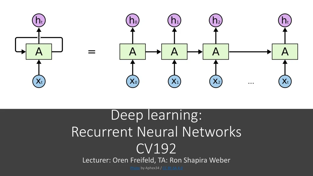
1. Deep learning: Recurrent Neural NetworksCV192 Lecturer: Oren Freifeld, TA: Ron Shapira Weber Photo by Aphex34 / CC BY-SA 4.0

2. Contents • Review of previous lecture – CNN • Recurrent Neural Networks • Back propagation through RNN • LSTM

3. Example – Object recognition and localization [Andrej Karpathy Li Fei-Fei, (2015): Deep Visual-Semantic Alignments for Generating Image Descriptions]

4. MLP with one hidden layer [Lecun, Y., Bengio, Y., & Hinton, G. (2015)]

5. How big should our hidden layer be? https://cs.stanford.edu/people/karpathy/convnetjs/demo/classify2d.html

6. Convolution • Discrete: kernel Convolution: matrix*kernel http://deeplearning.net/software/theano/tutorial/conv_arithmetic.html

7. . CNN – Convolutional Layer Filters learned by AlexNet (2012) 96 convolution kernels of size 11x11x3 learned by the first convolutional layer on the 224x224x3 input images (ImageNet) Krizhevsky, A., Sutskever, I., & Hinton, G. E. (2012).

8. . CNN – Pooling Layer • Reduce the spatial size of the next layer http://cs231n.github.io/convolutional-networks/

9. . CNN – Fully connected layer • Usually the last layer before the output layer (e.gsoftmax)

10. . Feature Visualization • Visualizing via optimization of the input: • Colah, etal., "FeatureVisualization", Distill, 2017.

11. Recurrent Neural Networks

12. Sequence modeling Examples: Video frame-by-frame classification Image classification Image captioning Sentiment analysis Machine translation http://karpathy.github.io/2015/05/21 /rnn-effectiveness/

13. DRAW: A recurrent neural network for image generation [Gregor, et al., (2015) DRAW: A recurrent neural network for image generation]

14. . Recurrent Neural Networks vsFeedforward Networks

15. . Recurrent Neural Networks Gradient flow

16. . Recurrent Neural Networks • Back propagation “through time”: • Chain rule application: • And: • = • where

17. . Recurrent Neural Networks • Truncated Back propagation • “through time”: • Break every K steps. • Forward propagation stays the same. • Downside?

18. . Recurrent Neural Networks • Example: RNN which predicts the next character • The corpus (vocabulary): • {h,e,l,o} • “one-hot” vectorization: h =

19. . Recall the vanishing gradient problem… Sigmoid Function: • when

20. . Gradient behavior in RNN • Let’s look at the gradient w.r.t. : Where: • when

21. Vanishing / exploding gradient • Optimization becomes tricky when the computational graph becomes extremely deep. • Suppose we need to repeatedly multiply by a weight matrix • Suppose that has an eigendecomposition • Any eigenvalues that are not near an absolute value of 1 will either explode if or vanish if . [Example from: Goodfellow, I., Bengio, Y., Courville, A., & Bengio, Y. (2016). Deep learning (Vol. 1). ]

22. . Vanishing / exploding gradient • On a more intuitive note, we working with a sequence of length t we have t copies of our network • On the scaler case, we backpropagate our gradient through t times until we reach . • If our gradient will explode • If our gradient will vanish.

23. . Long Short Term Memory (LSTM) • Long Short Term Memory networks (LSTM) are designed to counter the vanishing gradient problem. • They introduce the “cell state” () parameter which allows for almost uninterrupted gradient flow through the network. • The LSTM module is composed of four gates (layers) that interact with one another: • Input gate • Forget gate • Output gate • t gate [Hochreiter, S., & Schmidhuber, J. (1997). Long short-term memory]

24. . LSTM vs regular RNN The repeating module in an LSTM contains four interacting layers. The repeating module in a standard RNN contains a single layer. http://colah.github.io/posts/2015-08-Understanding-LSTMs/

25. . LSTM • The Cell state holds information about previous state – memory cell. http://colah.github.io/posts/2015-08-Understanding-LSTMs/

26. . LSTM – Gradient Flow Chen, G. (2016). A Gentle Tutorial of Recurrent Neural Network with Error Backpropagation

27. . Input gate • The input gate layer decides what information should go to the current state w.r.t. the current input ( • When we ignore the current time step. http://colah.github.io/posts/2015-08-Understanding-LSTMs/

28. . (tanh) gate • Creates the current state http://colah.github.io/posts/2015-08-Understanding-LSTMs/

29. . Forget Gate • The forget gate layer decides what information to discard from the previous state w.r.t. the current input () • It scales input with a sigmoid function. • When we “forget” the previous state. http://colah.github.io/posts/2015-08-Understanding-LSTMs/

30. . Output Gate • The output gate layer filters the cell state . • It decides what information goes “out” of the cell and what remains hidden from the rest of the network. http://colah.github.io/posts/2015-08-Understanding-LSTMs/

31. . LSTM Where is the next hidden state. http://colah.github.io/posts/2015-08-Understanding-LSTMs/

32. . LSTM Summary • LSTM solves the problem of vanishing gradient by introducing the memory cells - which is mostly defined by addition and element-wise multiplication operators. • The gates system filters what information we keep from the previous states and what information to add from the current state.

33. . Increasing model memory • Increasing memory: • Increasing the size of the hidden layer increases the model size and computation quadratically (are fully-connected)

34. . Increasing model memory • Adding more hidden layers increases the model capacity while computation scales linearly. • Increases representational power via non-linearity.

35. . Increasing model memory • Adding depth through ‘time’. • Does not increase memory. • Increases representational power via non-linearity.

36. . Neural Image Caption Generation with Visual Attention [Xu et al.,(2015) Show and tell: A neural image caption generator]

37. . Neural Image Caption Generation with Visual Attention [Xu et al.,(2015) Show and tell: A neural image caption generator]

38. . Neural Image Caption Generation with Visual Attention [Xu et al.,(2015) Show and tell: A neural image caption generator]

39. . Neural Image Caption Generation with Visual Attention • Word generation conditioned on: • Context vector (CNN features) • Previous hidden state • Previously generated word [Xu et al.,(2015) Show and tell: A neural image caption generator]

40. Shakespeare http://karpathy.github.io/2015/05/21/rnn-effectiveness/

41. Visualizing the predictions and the “neuron” firings in the RNN http://karpathy.github.io/2015/05/21/rnn-effectiveness/

42. Visualizing the predictions and the “neuron” firings in the RNN http://karpathy.github.io/2015/05/21/rnn-effectiveness/

43. Visualizing the predictions and the “neuron” firings in the RNN http://karpathy.github.io/2015/05/21/rnn-effectiveness/

44. [http://norman-ai.mit.edu/[

45. [http://norman-ai.mit.edu/[

46. [http://norman-ai.mit.edu/[

47. . Summary • Deep learning is a field of machine learning that uses artificial neural network in order to learn representations in an hierarchical manner. • Convolutional neural achieved state-of-the-art results in the field of computer vision by • Reducing the number of parameters via shard weights and local connectivity. • Using an hierarchal model. • Recurrent neural network are used for sequence modelling. The vanishing gradient problem is address by a model called LSTM.

48. . Thanks!