Download
1 / 41
410 likes | 569 Views
Proportion Testing. October 2, 2009 Statistics Symposium. Outline. What we are covering and what we are not covering today Virtual Scavenger Hunt Statistical Decisions and Risk Six Sigma DMAIC application The Business Approach Hypothesis Test Approach Understanding Distributions

E N D
Proportion Testing October 2, 2009 Statistics Symposium
Outline • What we are covering and what we are not covering today • Virtual Scavenger Hunt • Statistical Decisions and Risk • Six Sigma DMAIC application • The Business Approach • Hypothesis Test Approach • Understanding Distributions • Sample Size • Test of Independence • Example 1: Regulatory Compliance Documentation • Example 2: Workload Balance (Productivity) • References and Web Sites • Q&A
Continuous Data Hypothesis Tests: What we are covering? 1 sample t-test : Δ mean from known test mean One Way ANOVA : At least 1 sample mean Δ between 3 or more samples 2 sample t-test: Δ mean between 2 independent sample means Kruskal Wallis & Mood’s Median: At least 1 sample median Δ between 3 or more samples Paired t-test: Δ mean between 2 dependent sample means F-test, Levene’s test, & Bartlett’s test: At least 1 sample standard deviation Δ between 3 or more samples Correlation/Regression/DOE: 2 or more factors are correlated/ Predictor affects the sampled process Attribute Data 1 proportion test: A sample proportion Δ against a known value 2 proportion test: Proportions from the two samples are different Chi Square test: At least one sample proportion Δ from others:
Scavenger Hunt • Find another person who can sign off on these statements. Each person can only sign once. • 1.Has used Chi-Square or Proportion Test • 2.Has more than $50 on them • 3.Used Minitab to determine sample size • 4.Worked on a project with a value proposition >$1 million • 5.Knows Chris Connors' middle name • 6.Has more than three children • 7.Has met a movie star or celebrity (and was not arrested) • 8.Knows the difference between a confidence interval and a confidence level • 9.Knows what a quark or a fantod is • 10. Has more than one academic degree, license or certification
Statistical Decision: Setting up your risk level • Type I and II errors • There are two kinds of errors that can be made in significance testing: • a true null hypothesis can be incorrectly rejected and • a false null hypothesis can fail to be rejected. The former error is called a Type I error and the latter error is called a Type II error. These two types of errors are defined in the table. The probability of a Type I error is designated by the Greek letter alpha (a) and is called the Type I error rate; the probability of a Type II error (the Type II error rate) is designated by the Greek letter beta (ß). A Type II error is only an error in the sense that an opportunity to reject the null hypothesis correctly was lost. It is not an error in the sense that an incorrect conclusion was drawn since no conclusion is drawn when the null hypothesis is not rejected.
Define Measure Control Analyze Improve Six Sigma DMAIC method: Hypothesis Tests • Six Sigma DMAIC method has 5 phases: • Define Opportunity/Problem • Measure Performance • Analyze Process and Performance • Improve Process and Performance • Control Process and Performance • I typically use this diagram to depict the continuous focus of measurement in the Six Sigma method by placing Measure in the center of the DMAIC method.
6S Black Belt Level of Cognition for Hypothesis Testing *1= learned, 2= know, 3 = used, 4 = taught
6S BB Level of Cognition for Hypothesis Testing *1= learned, 2= know, 3 = used, 4 = taught
The Business Approach Potential Root Causes Identified Statistical Problem Business Problem Statistical Problem Proportion Tests Decision • When we want to make a statistical comparison of a discrete variable with a target, or between two discrete variables, Proportion Tests should be used. Business Solution Statistical Solution Root Causes Verified
Selecting the Right Statistical Tool Y Discrete Continuous Proportion Tests t test ANOVA DOE Discrete X Logistic Regression Correlation Regression Continuous
Comparing Proportions 1 Sample 2 Samples More Than 2 Samples 1 ProportionTest 2 ProportionTest Chi-SquareTest Tests of Proportion Determine if a statistically significant difference of proportion exists between: - A sample and a target - Two independent samples - Two samples or less Use samples to make inferences about population proportions
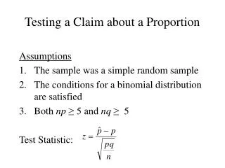
Proportion Test Approach • State the null and alternative hypotheses • Null H0 P1 = P2 Number of tails = 2 • P1 - P2 0 Number of tails = 1 • P1 - P2 0 Number of tails = 1 • Alternatives Ha P1 - P2 0 P1 P2 Number of tails = 1, left or right • P1- P2 0 • P1- P2 0 • 2. Formulate an analysis plan: 1 Proportion to known value (z) or 2 Proportions test • 3. Analyze sample data • Independence Test: Fisher’s, Barnard’s, G-Test • Pooled sample proportion to compute standard error • P value for test statistic • 4. Interpret results: for a statistical decision (hopefully a business decision, not not always) • If P is low, H0 must be no go
Useful Discrete Distributions • Binomial distribution for: • The number X of successes (or failures!) in n trials when p is the chance of success (or failure!) or each trial. • Examples: • number X of faulty expense reports out of n=100 submitted in a particular month, when the faulty expense report rate typically runs at p=0.03 (i.e., 3%) • number of voters out of a random sample of n=800 expressing approval of the President’s performance, when the approval rating in the entire population of voters is p=0.42 (i.e., 42%) • X is discrete: it must be one of 0, 1, 2, … , n
Binomial - key facts Useful fact: has approximately a normal distribution when n is large (more than 25 or 30) and np and n(1-p) are not too small (say >5).
Sample Size • General Guidelines (if not followed, test may not run): • Each Sample includes at least 10 failures and 10 successes (some texts say 5) • The sample is from a population 10 x the sample • Use Minitab sample size calculator • Use TI 83 or TI 84 Graphing Calculator (see web)
Hypothesis testing - terms • Null hypothesis (H0) – e.g., µ1 = µ2 - this is the hypothesis to be tested and should be in the form of a true/false statement . This hypothesis states that there is NO DIFFERENCE between the data sets or samples or populations. Null hypotheses are never accepted – we either reject them or fail to reject them. The null hypothesis has PRIORITY and should not be rejected unless there is strong statistical evidence to do so. • Alternate hypothesis (H1, HA) – e.g., µ1 ≠ µ2 - the alternative to the null hypothesis – states that there IS A DIFFERENCE between the data sets or populations. • Type 1 error – rejecting the null hypothesis when it is really true – e.g., “convicting the innocent” • Type 2 error – failing to reject the null hypothesis when it really is false – e.g., “letting the guilty go free” • Level (or size) of a test = Alpha (α) – is the probability of a type 1 error – default = 5% • Beta (β) – is the probability of a type 2 error – default = 10% • Power of a test or power – is the probability of correctly rejecting a false null hypothesis. Since β is the probability of a type I error, power is calculated by the formula (1 - β). Power = (1 - β) when the null hypothesis is false. The default value for power is 90%This means that you have an 90% chance of finding a difference when you really want to find it. • Critical region (rejection region) – set of values of the test statistic that cause the null hypothesis to be rejected. If the test statistic falls into the rejection region, the null hypothesis is rejected.
Hypothesis testing steps • State the null hypothesis H0 and the alternate hypothesis HA (e.g., the mean incomes of college graduates does not equal that of other people) • Choose the level of significance, alpha (α default = 0.05) and the sample size (default n = 25) • Choose the appropriate statistical techniques (t test, Chi-square, etc.,) and test statistic (e.g., mean) • Collect the data and calculate the sample value of the test statistic • Calculate the p value based on the test statistic and compare it with alpha (α = 0.05) • Make a statistical decision – if p is greater than or equal to alpha, fail to reject the null hypothesis. If the p value is less than alpha, reject the null hypothesis.
Hypothesis tests are either one tailed or two tail tests Reject H0 Reject H0 Fail to Reject H0 Fail to Reject H0 One tail test - Answers only ONE question - is the test statistic less than or greater than the known distribution 1% or 5% significance level Fail to Reject H0 Reject H0 Reject H0 Two tailed test – Only asks if the test statistic is different from the known distribution – HA usually has “not equal to” in the wording 2.5% significance level 2.5% significance level
Clinical Testing One-tailed example by hand • The “Feel Good” Drug company has discovered a new drug which prevents acne. Since the market for skin care products is larger for woman than men, the company would like to be able to show a treatment advantage for women vs men. The company statistician chooses a simple random sample of 110 women and 207 men from a population of 100,000 healthy volunteers. After 6 months, 48% of women had no acne, vs 61% of men. Can the company claim a benefit for women vs men at the 0.01 level of significance? • What are the hypotheses? • Calculate the pooled sample proportion and the Standard Error and consult the z-score statistic • What do the results tell us?
Clinical Testing One-tailed example by hand • 1) What are the hypotheses? • Ho - P1 = P2 • Ha – P1 < > P2 • The null hypothesis will be rejected if the proportion of women developing acne (p1) is substantially smaller than the proportion of men developing acne (p2) • Calculate the pooled sample proportion and the Standard Error and consult the z-score statistic: • P = (p1 * n1 + p2 * n2)/(n1 + n2) • = [(0.48 *110) + (0.61 * 207)]/(110 + 207) • = 52.8 + 126.3 / 317 • = 0.564 • SE = sqrt { p * (1 - p) * [(1/n1) + (1/n2)]} • = [ 0.564 * 0.436 * (1/110 + 1/207) • = sqrt 0.245 * (0.009 + 0.005) • = 0.058 • Z = (p1 - p2)/SE = (0.48 - 0.61) / 0.058 • = -2.24 • Since this is a one tailed test, the P value is the probability that the z-score is • less than -2.24. The Normal distribution calculator for P (z < -2.24) = 0.013 • P value = 0.013. Since 0.013 is greater than the chosen significance level (0.01), • WE FAIL TO REJECT THE NULL HYPOTHESIS – THERE IS NO STATISTICAL DIFFERENCE BETWEEN THE POPULATIONS
Test of Independence • Fisher’s Exact Test is most commonly used for 2 x 2 tables to determine if there is a nonrandom relationship between two categorical variables. Fisher’s calculates conditional probability for the observed row and column matrix. • Fisher’s exact test in Minitab: Rows: adverse Columns: drug new old All n 90 80 170 y 210 120 330 All 300 200 500 Cell Contents: Count Fisher's exact test: P-Value = 0.0265193
The Business Approach Potential Root Causes Identified Statistical Problem Business Problem Statistical Problem 1-Proportion Test Decision Business Solution Statistical Solution Root Causes Verified
Regulatory Compliance Documentation Example • A Black Belt is studying the company’s ability to get regulatory compliance documentation to the record center with in 5 days from project completion. • What is the binomial characteristic? • A random sample of 130 project documentation records showed that 74 of them met the 5 day deadline. • The business was heard saying “at least we’re over the half way mark!” • Test the hypothesis at 95% confidence that more than 50% of engagements met the deadline. • What is the Null Hypothesis?
Regulatory Compliance Documentation Example - Hypothesis • Ho : The proportion of compliance documentation filed at the record center on time is 50% (interim target value). • Ha : The proportion of external work papers filed at the record center on time is greater than 50%. • Note: Typically the alternative is stated as “there is a difference.” • Why does this example state “greater than?”
Compliance Documentation Example – Minitab Commands • Tool Bar Menu > Stat > Basic Statistics > 1 Proportion Analysis target
Compliance Documentation Example – Minitab Results Test and CI for One Proportion Test of p = 0.5 vs p > 0.5 95% Lower Exact Sample X N Sample p Bound P-Value 1 74 130 0.569231 0.493309 0.068 What’s our interpretation?
Regulatory Compliance Documentation Sample Size • Power and Sample Size • Test for Two Proportions • Testing proportion 1 = proportion 2 (versus <) • Calculating power for proportion 2 = 0.7 • Alpha = 0.05 • Sample Target • Proportion 1 Size Power Actual Power • 0.6 388 0.9 0.900148 • 0.6 281 0.8 0.800923 • The sample size is for each group. • Is the sample size a concern?
The Business Approach Potential Root Causes Identified Statistical Problem Business Problem Statistical Problem 2-Proportion Test Decision Business Solution Statistical Solution Root Causes Verified
Analysis of Proportions for Workload BalanceJack Lairdieson, MBB, Vanguard Total Region 5 Region 6 Region 3 Region 1 Region 3 Region 2 Interpret as an Interval Plot for Multiple Proportions
Workload Balance Example The Workload Balance (WLB) metrics were being discussed at a regional meeting. The Region 1 representative scoffed at the Region 2 representative that the Region 2’s “In-range” WLB performance metrics were at the “bottom of the barrel”. The Region 2 representative quickly responded, “Really, Region 1 is no better than Region 2.”Once back to the office the concerned Region 1 representative gave the following Workload Balance data to a Black Belt.WLB Stats In-Range Staff Region 1 663 1411 Region 2 141 353Should Region 1 be concerned about his conclusion? What is the null hypothesis?
Workload Balance Example - Hypothesis • Ho : The proportion of Region 1 “In-Range” staff is equal to the proportion of Region 2 “In-Range” staff. • Ha : The proportion of Region 1 “In-Range” staff is not equal to the proportion of Region 2 “In-Range” staff. • or • Ha : The proportion of Region 1 “In-Range” staff is greater than the proportion of Region 2 “In-Range” staff.
Workload Balance Example – Minitab Commands • Tool Bar Menu > Stat > Basic Statistics > 2 Proportion • Analysis through MINITAB™
Workload Balance Example – Minitab Results Session Window Output Test and CI for Two Proportions Sample X N Sample p 1 663 1411 0.469880 2 141 353 0.399433 Difference = p (1) - p (2) Estimate for difference: 0.0704461 95% lower bound for difference: 0.0223190 Test for difference = 0 (vs > 0): Z = 2.41 P-Value = 0.008 What’s our interpretation? What Hypothesis did we choose to test? Is the sample size a concern?
Sample Size: Minitab • Testing proportion 1 = proportion 2 (versus >) • Calculating power for proportion 2 = 0.399 • Alpha = 0.05 • Sample Target • Proportion 1 Size Power Actual Power • 0.469 857 0.9 0.900072 • 0.469 619 0.8 0.800094 • The sample size is for each group.
References • Fisher RA (1925). Statistical Methods for Research Workers. Oliver and Boyd, Edinburgh • Barnard GA (1945). A new test for 2 x 2 tables. Nature 156:177 • Chan I (1998) Exact tests of equivalence and efficacy with non-zero lower bound for comparative studies. Statistics in Medicine 17, 1403-1413 • Mehta CR and Senchaudhuri P (2003). Conditional versus unconditional tests for comparing two binomials. Cytel Software. • Web Sites: • http://www.minitab.com/support/documentation/answers/ • SampleSize2p.pdf • www.statsoft.com/textbook/stathome • http://sofia.fhda.edu/gallery/statistics/lessons/lesson10-2
Six Sigma Links Six Sigma Motorola, Inc. - Motorola University Six Sigma - What is Six Sigma? i Six Sigma - Six Sigma Quality Resources for Achieving Six Sigma Results General Electric : Our Company : What is Six Sigma? Quality American Society for Quality - ASQ TQM Virtual CoursePack SPC Press - Home Statistics http://www.statsoft.com/textbook/stathome.html Penn State Statistical Education Resource Kit--Overview of Statistics Data Statistics Video Course The Sofia Open Content Initiative - Elementary Statistics Resource: Learning Math: Data Analysis, Statistics, and Probability Lean Six Sigma Kaizen and Lean Manufacturing Consulting: Gemba Research - | Kaizen Products Conquering Complexity, Fast Innovation, Lean Six Sigma Quality. George Group Consulting Six Sigma Training Book LEAN.org - Lean Enterprise Institute| Lean Production| Lean Manufacturing| LEI| Lean Services| Lean Enterprise Training Course| Lean Consumption| Lean Resources| Lean Experts| Lean Healthcare| Lean in Healthcare| Training on Lean Manufacturing| Lean Business Excel Statistics Add on http://www.qimacros.com/