Download
1 / 31
330 likes | 545 Views
Hypothesis Testing: One Sample Mean or Proportion. Introduction, Section 10.1 -10.3 Testing a Mean, Section 10.5. Hypothesis: A Statement about a Population Parameter. The Labor Department makes a statement Mean annual earnings of white men in 1968 was $8000 (quantitative variable)

E N D
Hypothesis Testing: One Sample Mean or Proportion Introduction, Section 10.1 -10.3 Testing a Mean, Section 10.5
Hypothesis: A Statement about a Population Parameter • The Labor Department makes a statement • Mean annual earnings of white men in 1968 was $8000 (quantitative variable) • A food company claims • The boxes contain 16 ounces of cereal (quantitative variable) • Advertising firm states that • 70% of customers like the new package design (qualitative variable) it is proposing PP 2
Null and Alternative Hypotheses • Claim being made is the null hypothesis • H0: = $8000 (Labor Dept. statement) • H0: = 16.0 ounces (Desired weight if machine is working correctly) • H0: = 0.70 (Ad firm) • This statement remains unless a challenger can refute it • The alternative hypothesis is a second statement that contradicts the null hypothesis PP 2
Null and Alternative Hypotheses • In this case, • H1: $8000 • Annual earnings are not equal to $8000 • H1: 16 ounces • The process is not in control • H1: 0.70 • The proportion of customers who like the new design is different from 70% PP 2
The Research Challenge • Use sample data to decide on the validity of the null hypothesis • Consider H0: = $8000 (Annual earnings of white men in 1968) • Obtain a random sample of men from 1968 • Use National Longitudinal Studies • Sample size is n = 1,976 • Known population standard deviation, = 4191.20 • Standard error of the sampling distribution • = 94.28 • The sample is so large that we can fall back on the CLT • Confident that the sampling distribution of the mean is approximately normal PP 2
Rationale • We compare the mean of the sample with the hypothesized population mean, = 8000 • Is the difference between the sample mean and the hypothesized mean (sample mean – 8000) “small” or “large” ? • A “small” difference • Suggests that the sample may be drawn from a population with a mean of 8000 • The null hypothesis can not be rejected • A “large” difference • Suggests that it is unlikely that the sample came from a population with a mean of 8000 • The sample appears to be drawn from a population with a mean other than 8000 • We reject the null hypothesis • Such a test result is said to be statistically significant PP 2
Rationale • How can we decide whether the difference between the sample mean and the hypothesized mean (sample mean – 8000) is “small” or “large”? • Consider how the distribution of sample means would look if the null hypothesis was true • “Under the null hypothesis” • Consider the claim to be correct for the moment PP 2
Sampling Distribution of Sample Means, Normally Distributed Under the Null Hypothesis • We know what to expect if the null H0 is true • 95.44% of the sample means ( ) lie within 2 standard errors, , of the population mean PP 2
Statistical Decision Approaches • Critical value • Establish boundaries beyond which it is unlikely to observe the sample mean if the null hypothesis is true • P-value • Express the probability of observing our sample mean or one more extreme if the null hypothesis is true • Approaches yield same results PP 2
Types of Error • Consider a criminal trial by jury in the US • The individual on trial is either innocent or guilty • Assumed innocent by law • After evidence is presented, the jury finds the defendant either guilty or not guilty PP 2
Two Types of Error PP 2
Hypothesis Testing • All statistical hypotheses consist of • A null hypothesis and an alternative hypothesis • These two parts are constructed to contain all possible outcomes of the experiment or study • The null hypothesis states the null condition exists • There is nothing new happening, the old theory is still true, the old standard is correct and the system is in control • The alternative hypothesis contains the research challenge or what must be demonstrated • The new theory is true, there are new standards, the system is out of control, and/or something is happening PP 2
Null and Alternative Hypotheses • The null and the alternative hypotheses refer to population parameters • Never to sample estimates • This is correct: H0: = 8000 This is WRONG: H0: = 8000 • Why? PP 2
Null Hypothesis • The null hypothesis contains the equality sign • Never put the equality sign in the alternative hypothesis • Null hypotheses usually do not contain what the researcher believes to be true • Typically researchers wish to reject the null hypothesis • Remember the term “null” • The null hypothesis typically implies • No change, no difference, and nothing noteworthy has happened PP 2
Alternative Hypothesis • The burden of proof is placed in the alternative hypothesis • A claim is made • H0: = 8000 • I do not believe the claim • The alternative hypothesis states my challenge • H1: 8000 • I must demonstrate that the claim is false • This alternative is called a two tail or two sided alternative • Want to know if the true mean is higher than or lower than the claim • Unless the sample contains evidence that allows me to reject the null hypothesis, the original claim stands as valid • Form the alternative hypothesis first, since it embodies the challenge PP 2
Specify the Level of Significance: The Risk Of Rejecting A True Null Hypothesis • How much error are you willing to accept? • The significance level of the test is the maximum probability that the null hypothesis will be rejected incorrectly, a Type I error • Use to designate the risk and we set = 0.05, 0.02, 0.01 by convention • When possible, set the risk of that we want • Do this in studies for which we determine the appropriate sample size PP 2
Sampling Distribution of Sample Means, Normally Distributed .95 do not reject ? ? ? ? Z Form the Rejection Region: Critical Values • Critical values divide the sampling distribution under the null hypothesis into a rejection and a non-rejection area • Set ⍺ = 0.05, 2-sided test (0.05/2 = 0.025) • The blue lines are the boundaries • Sample means • Z values .025 reject .025 reject PP 2
Do Not Reject H 0 Reject H Reject H 0 0 1-a –z.025 +z.025 -1.96 1.96 Determine Specific Critical Values Standard Normal Distribution • Need the Z value such that 5% of standardized values lie in the two tails • 2.5% lies in each tail • Designate this unknown Z value as Z.05/2 or Z.025 • If .025 lies in the tail of the distribution, then 0.5000 - 0.025 = 0.4750 lies between the mean of 0 and this unknown Z value • Standard normal tables • Read from the probabilities out to the Z values, we find a value of 1.96 .4750 .025 0 PP 2
Rationale of Test • 95% of Z values lie within 1.96 standard deviations from the mean • When the null hypothesis is true • 95% of sample means will lie within 1.96 standard errors of the population mean • 5% of sample means will lie beyond 1.96 standard errors of the population mean • Argument by contradiction • View 5% as a small probability • If a sample means falls in the 5% region • We are skeptical about null PP 2
Determine the Correct Test Statistic • Test Statistic is a formula that summarizes sample information • Test Statistic =(sample statistic – claim about population parameter)/ standard error • Is the population standard deviation, σ, known? • If yes, use Z values • If no, use the student t distribution PP 2
State the Decision Rule (DR) • DR: if (-Z/2 < Z test statistic < Z/2) do not reject the null hypothesis, two sided test • If ⍺ = 0.05, Z.025 = ± 1.96 • If (-1.96 ≤ Z test statistic ≤ 1.96) do not reject • DR : if (-tn-1,/2 < t - test statistic < tn-1, /2) do not reject the null hypothesis PP 2
Statistical Decision and Conclusions • Reject or do not reject the null hypothesis • This is the statistical decision • Online homework refer to this as the conclusion • State the conclusions in terms of the problem • Simple statement in English • What is the business decision? • What is the economic policy conclusion? PP 2
Problem - Income in the 1960s • Consider our example • H0: = $8000H1: $8000 • Let = .05 Z.025 = 1.96 • DR: if (-1.96 ≤ Z test statistic ≤ 1.96) do not reject • The sample mean, , =$7814.10 • Sample size is n = 1,976 • Known population standard deviation, = 4191.20 • Standard error of the sampling distribution • = 94.28 PP 2
Sampling Distribution of Sample Means, Normally Distributed .95 do not reject 7814.1 -1.97 -1.96 1.96 Z Calculate the Test Statistic • Convert the sample mean into the test statistic, a Z test • How far does 7814.10 lie from 8000 in terms of the number of standard errors? • Z = (7814.1-8000)/94.28 = -1.97 • Reject the null hypothesis at a 5% level of significance, two-tailed test PP 2
Change the Level of Significance • Lower the risk of a Type I error • Let =0 .01, two sided test • Z.01/2 = Z.005 = 2.58 • DR: if (-2.58 ≤ Z test statistic ≤ 2.58) do not reject • Test Statistic = -1.97 • No evidence to reject • Set before any statistical tests are performed PP 2
Do Not Reject H 0 Reject H Reject H 0 0 1-a –z.005 +z.005 -2.58 2.58 Lower the Level of Significance to 0.01 • Let =0 .01, two sided test • Z.01/2 = Z.005 • If .005 lies in the tail of the distribution, then 0.5000 - 0.005 = 0.4950 lies between the mean of 0 and this unknown Z value • Standard normal tables • Read from the closest probabilities out to the Z values, we find a value of 2.57 or 2.58 .4950 .005 PP 2
Standard Normal Distribution PP 2 Between 2.57 and 2.58
Student t Distribution Z.005 = 2.5758 = 2.58 PP 2
Online Homework - Chapter 10 Intro to Hypothesis Testing and Testing a Mean • CengageNOW second assignment • CengageNOW: Chapter 10 Intro to Hypothesis Testing • CengageNOW third assignment • CengageNOW: Chapter 10 Testing a Mean PP 2