Download
1 / 105
1.09k likes | 1.4k Views
Vectors. Vectors: notations. A vector in a n-dimensional space in described by a n-uple of real numbers. x 2. B 2. B. A. A 2. x 1. A 1. B 1. Vectors: sum. The components of the sum vector are the sums of the components. x 2. C 2. C. B 2. B. A. A 2. A 1. B 1. C 1. x 1.

E N D
Vectors: notations • A vector in a n-dimensional space in described by a n-uple of real numbers x2 B2 B A A2 x1 A1 B1
Vectors: sum • The components of the sum vector are the sums of the components x2 C2 C B2 B A A2 A1 B1 C1 x1
Vectors: difference • The components of the sum vector are the sums of the components x2 B2 B A C2 A2 C A1 C1 B1 x1 -A
Vectors: product by a scalar • The components of the sum vector are the difference of the components x2 C2 3A A A2 A1 C1 x1
Vectors: Norm • The most simple definition for a norm is the euclidean module of the components x2 A2 A A1 x1
Vectors: distance between two points • The distance between two points is the norm of the difference vector x2 B2 B A C2 A2 C A1 C1 B1 x1 -A
Vectors: Scalar product • The components of the sum vector are the sums of the components x2 B2 B A A2 θ A1 B1 x1
Vectors: Norm and scalar product • The components of the sum vector are the sums of the components
Vectors: Definition of an hyperplane In R2 , an hyperplane is a line A line passing through the origin can be defined with as the set of the vectors that are perpendicular to a given vector W x2 W x1
Vectors: Definition of an hyperplane In R3 , an hyperplane is a plane A plane passing through the origin can be defined with as the set of the vectors that are perpendicular to a given vector W x3 W x1 x2
Vectors: Definition of an hyperplane In R2 , an hyperplane is a line A line perpendicular to W and whose distance from the origin is equal to b is defined by the points whose scalar vector with W is equal to b -b>0 x2 X -b/|W| W x1
Vectors: Definition of an hyperplane In R2 , an hyperplane is a line A line perpendicular to W and whose distance from the origin is equal to b is defined by the points whose scalar vector with W is equal to b x2 X W x1 b/||W|| -b<0
Vectors: Definition of an hyperplane In Rn , an hyperplane is defined by
An hyperplane divides the space A <AW>/||W|| x2 X <BW>/||W|| -b/||W|| W x1 B
Distance between a hyperplane and a point A <AW>/||W|| x2 X <BW>/||W|| -b/||W|| W x1 B
Distance between two parallel hyperplane -b’/||W|| x2 W x1 -b/||W||
Aim We want to maximise the function z = f(x,y) subject to the constraints g(x,y) = c (curve in the x,y plane) 9/10/2014 20
Simple solution Solve the constraint g(x,y) = c and express, for example, y=h(x) The substitute in function f and find the maximum in x of f(x, h(x)) Analytical solution of the constraint can be very difficult
Geometrical interpretation The level contours of f(x,y) are defined by f(x,y) = dn 22
Lagrange Multipliers Suppose we walk along the contour line with g = c. In general the contour lines of f and g may be distinct: traversing the contour line for g = c we cross the contour lines of f. While moving along the contour line for g = c the value of f can vary. Only when the contour line for g = c touches contour lines of ftangentially, we do not increase or decrease the value of f - that is, when the contour lines touch but do not cross. 23
Gradient of a curve Given a curve g(x,y) = c the gradient of g is: Consider 2 points of the curve: (x,y); (x+εx, x+εy), for small ε (x+εx, x+εy) (x,y)
Gradient of a curve Given a curve g(x,y) = c the gradient of g is: Since both points satisfy the curve equation: For small ε, ε is parallel to the curve and, consequently, the gradient is perpendicular to the curve (x+εx, x+εy) (x,y) ε grad (g)
Lagrange Multipliers The point on g(x,y)=c that Max-min-imize f(x,y) the gradient of f is perpendicular to the curve g, otherwise we should increase or decrease f by moving locally on the curve So, the two gradients are parallel for some scalar λ (where is the gradient). 27
Lagrange Multipliers • Thus we want points (x,y) where g(x,y) = c and • , • To incorporate these conditions into one equation, we introduce an auxiliary function (Lagrangian) • and solve • . 28
Recap of Constrained Optimization • Suppose we want to: minimize/maximize f(x) subject to g(x) = 0 • A necessary condition for x0 to be a solution: • a: the Lagrange multiplier • For multiple constraints gi(x) = 0, i=1, …, m, we need a Lagrange multiplier ai for each of the constraints - -
Constrained Optimization: inequality • We want to maximize f(x,y) with inequality constraint g(x,y)£c. • The search must be confined in the red portion (gradient of a function points towards the direction along which it increases) g(x,y) ≤ c
Constrained Optimization: inequality • maximize f(x,y) with inequality constraint g(x,y)£c. • If the gradients are opposite (l<0) the function increases in the allowed portion The maximum cannot be on the curve g(xy)=c • Maximum is on the curve only if l>0 g(x,y) ≤ c f increases, l<0
Constrained Optimization: inequality • Minimize f(x,y) with inequality constraint g(x,y)£c. • If the gradients are opposite (l<0) the function increases in the allowed portion • Minimum is on the curve only if l<0 g(x,y) ≤ c f increases, l<0
Constrained Optimization: inequality • maximize f(x,y) with inequality constraint g(x,y)≥c. • If the gradients are opposite (l<0) the function decreases in the allowed portion • Maximum is on the curve only if l<0 g(x,y) ≥ c l<0 f decreases,
Constrained Optimization: inequality • Minimize f(x,y) with inequality constraint g(x,y)≥c. • If the gradients are opposite (l<0) the function decreases in the allowed portion • Minimum is on the curve only if l>0 g(x,y) ≥ c l<0 f decreases,
Karush-Kuhn-Tucker conditions with αi satisfying the following conditions: and The function f(x) subject to constraints gi(x) ≤or≥ 0 is max-minimized by opimizing the Lagrange function
Constrained Optimization: inequality • Karush-Kuhn-Tucker complementarity condition means that The constraint is active only on the border, and cancel out in the internal regions
Concave-Convex functions Concave Convex
Dual problem • If f(x) is a convex function Is solved by: From the first equation we can find x as a function of the ai These can be substituted in the Lagrangian function obtaining the dual Lagrangian function
Dual problem • The dual Lagrangian is concave: maximising it with respect to ai ,with ai>0, solve the original constrained problem. We compute ai as: Then we can obtain x by substituting using the expression of x as a function of ai
Dual problem:trivial example • Minimize the function f(x)=x2 with the constraint x≤-1 (trivial: x=-1) The Lagrangian is Minimising with respect to x The dual Lagrangian is Maximising it gives: a=2 Then subsituting, -1
Class 2 Class 1 What is a good Decision Boundary? • Consider a two-class, linearly separable classification problem • Many decision boundaries! • The Perceptron algorithm can be used to find such a boundary • Are all decision boundaries equally good?
Examples of Bad Decision Boundaries Class 2 Class 2 Class 1 Class 1
Large-margin Decision Boundary • The decision boundary should be as far away from the data of both classes as possible • We should maximize the margin, m Class 2 m Class 1
Finding the Decision Boundary • Let {x1, ..., xn} be our data set and let yiÎ {1,-1} be the class label of xi For yi=1 For yi=-1 y=1 y=1 So: y=1 y=-1 y=1 y=1 y=-1 Class 2 y=-1 y=-1 y=-1 m y=-1 Class 1
Finding the Decision Boundary • The decision boundary should classify all points correctly Þ • The decision boundary can be found by solving the following constrained optimization problem • This is a constrained optimization problem. Solving it requires to use Lagrange multipliers
Finding the Decision Boundary • The Lagrangian is • ai≥0 • Note that ||w||2 = wTw
Gradient with respect to w and b • Setting the gradient of w.r.t. w and b to zero, we have n: no of examples, m: dimension of the space
The Dual Problem • If we substitute to , we have Since • This is a function of ai only