Download

1 / 14
140 likes | 208 Views
Testing the Efficacy of Climate Forecast Maps as a Means of Communicating with Policy Makers Toru Ishikawa 1 , Anthony G. Barnston 2 , Kim A. Kastens 1,3 , Patrick Louchouarn 3,1 , and Chester F. Ropelewski 2

E N D
Testing the Efficacy of Climate Forecast Maps as a Means of Communicating with Policy Makers Toru Ishikawa1, Anthony G. Barnston2, Kim A. Kastens1,3, Patrick Louchouarn3,1, and Chester F. Ropelewski2 1 Lamont-Doherty Earth Observatory, Columbia University, Palisades, NY 10964 (ishikawa@ldeo.columbia.edu, kastens@ldeo.columbia.edu) 2 International Research Institute for Climate Prediction, Palisades, NY 10964 (tonyb@iri.columbia.edu, chet@iri.columbia.edu) 3 Department of Earth and Environmental Sciences, Columbia University, New York, NY 10027 (pl2065@columbia.edu) Presented at the Climate Prediction Applications Science Workshop FSU, Tallahassee FL 9-11 March 04
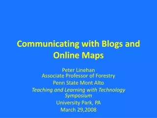
Figure 2. Probability forecast map of precipitation for Feb-Mar-Apr 2003
Question 1. The first map (Map 1) is a probability forecast map of precipitation for February-March-April 2003. The map was made in January 2003. It shows in color the probability that individual locations would have more or less precipitation than normal. Normal is defined as being in the center one-third of the years in a 30-year database. Above normal is defined as being in the wettest one-third of the years, and below normal is defined as being in the driest one-third of the years, in the 30-year database. The horizontal bar graphs shown on the colored areas indicate the probability of forecasts falling into, from top to bottom, the above normal, the normal, and the below normal categories. Suppose that you are given this forecast map (Map 1) in January 2003. Based on this map, how would you answer the following question: "Which area will receive a greater amount of total precipitation for this forecast period, Southern California or Washington State?" Please explain in a few sentences how you came to the answer (or the difficulty you had in trying to answer the question).
Fig. 5 Number of participants who correctly and incorrectly evaluated the maps.
Figure 3A. Probability forecast map of precipitation for Oct-Nov-Dec 2002.
Figure 3B. Observed precipitation map for Oct-Nov-Dec 2002.
The third pair of maps shows the above normal threshold (Map 3A) and the below normal threshold (Map 3B). The above normal threshold is the border between the normal category and the above normal category; the below normal threshold is the border between the normal category and the below normal category. These thresholds are used in making the forecast maps such as Map 1. Maps 3A and 3B cover the same 3-month period as for Map 1. Suppose that you are given Maps 3A and 3B, together with Map 1. Please complete the following statements about the probabilities of above normal and below normal precipitation at the two locations for this forecast period: (a) (i) Above normal: The probability is _____% that Charleston, South Carolina (denoted by C on Maps 3A and 3B), will receive more than _____ mm of precipitation. (ii) Below normal: The probability is _____% that Charleston, South Carolina, will receive less than _____ mm of precipitation. Please explain in a few sentences how you came to the answer (or the difficulty you had in trying to answer the question). (b) (i) Above normal: The probability is _____% that Phoenix, Arizona (denoted by P on Maps 3A and 3B), will receive more than _____ mm of precipitation. (ii) Below normal: The probability is _____% that Phoenix, Arizona, will receive less than _____ mm of precipitation. Please explain in a few sentences how you came to the answer (or the difficulty you had in trying to answer the question).
Imagine that you are the Secretary of Agriculture of the US and that this pair of forecast/observed maps is representative of the last 5 years of forecasts. Would you recommend that these forecasts be used to make decisions about what crops to plant? Circle one number from 1 to 5 below concerning your action: • strong recommendation for using the forecasts; (2) weak recommendation for using the forecasts; (3) no recommendation in either way; (4) weak recommendation for NOT using the forecasts; (5) strong recommendation for NOT using the forecasts.
Would you recommend using these forecasts? 1 - Strongly Recommend 2 - Weakly Recommend 3 – No Action 4 - Weakly Recommend against 5 - Strongly Recommend against
Preliminary Conclusions 1.Even these qualified and motivated students, in an elite master’s program aimed for prospective policy makers, failed to interpret some of the forecast maps as the map maker intended. 2.Specialists ability to understand complex Earth systems exceeds the ability of available communication tools to convey that understanding to policy makers and their non-specialist audiences. 3. The students understood observed precipitation maps easily, whereas they had more trouble understanding probability forecast maps. 4.It was particularly difficult for the students to make logical inference by referring to and integrating different aspects of climate forecasts. 5. Many (more than half) of the students were not inclined to rely on these types of climate forecasts for agriculture decision making.