Download
1 / 12
120 likes | 211 Views
Optimization with surrogates. Based on cycles. Each consists of sampling design points by simulations, fitting surrogates to simulations and then optimizing an objective. Zooming (This lecture) Construct surrogate, optimize original objective , refine region and surrogate.

E N D
Optimization with surrogates • Based on cycles. Each consists of sampling design points by simulations, fitting surrogates to simulations and then optimizing an objective. • Zooming (This lecture) • Construct surrogate, optimize original objective, refine region and surrogate. • Typically small number of cycles with large number of simulations in each cycle. • Adaptive sampling (Lecture on EGO algorithm) • Construct surrogate, add points by taking into account not only surrogate prediction but also uncertainty in prediction. • Most popular, Jones’s EGO (Efficient Global Optimization). • Easiest with one added sample at a time.
Design Space Refinement • Design space refinement (DSR): process of narrowing down search by excluding regions because • They obviously violate the constraints • Objective function values in region are poor • Called also Reasonable Design Space. • Benefits of DSR • Prevent costly simulations of unreasonable designs • Improve surrogate accuracy • Techniques • Use inexpensive constraints/objective. • Common sense constraints • Crude surrogate • Design space windowing Madsen et al. (2000) Rais-Rohaniand Singh (2004)
Radial Turbine Preliminary Aerodynamic Design Optimization Yolanda Mack University of Florida, Gainesville, FL Raphael Haftka, University of Florida, Gainesville, FL Lisa Griffin, Lauren Snellgrove, and Daniel Dorney, NASA/Marshall Space Flight Center, AL Frank Huber, Riverbend Design Services, Palm Beach Gardens, FL Wei Shyy, University of Michigan, Ann Arbor, MI 42nd AIAA/ASME/SAE/ASEE Joint Propulsion Conference & Exhibit 7-12-06
Radial Turbine Optimization Overview • Improve efficiency and reduce weight of a compact radial turbine • Two objectives, hence need the Pareto front. • Simulations using 1D Meanlinecode • Polynomial response surface approximations used to facilitate optimization. • Three-stage DSR • Determine feasible domain. • Identify region of interest. • Obtain high accuracy approximation for Pareto front identification.
Maximizeηts and MinimizeWrotor such that Optimization Problem • Objective Variables • Rotor weight • Total-to-static efficiency • Design Variables • Rotational Speed • Degree of reaction • Exit to inlet hub diameter • Isentropic ratio of blade to flow speed • Annulus area • Choked flow ratio • Constraints • Tip speed • Centrifugal stress measure • Inlet flow angle • Recirculation flow coefficient • Exit to inlet shroud radius
0 < β1 < 40 React > 0.45 Infeasible Region Feasible Region Range limit Phase 1: Aproximatefeasible domain • Design of Experiments: Face-centered CCD (77 points) • 7 cases failed • 60 violated constraints • Using RSAs, dependences determined for constraints • Variables omitted for which constraints are insensitive • Constraints set to specified limits
Feasible Region Infeasible Region Infeasible Region Feasible Region Feasible Regions for OtherConstraints • Two constraints limit a the values of one variableeach. • All invalid values of a third constraint lie outside of new ranges • Fourth constraint depend on three variables.
Refined DOE in feasible region • New 3-level full factorial design (729 points) using reduced ranges. • 498 / 729 were eliminated prior to Meanline analysis based on the two 3D constraints. • 97% of remaining 231 points found feasible using Meanlinecode.
1 – ηts Wrotor Use different surrogates to estimate accuracy • Five RSAs constructed for each objective minimizing different norms of the difference between data and surrogate (loss function). • Normp = 1,2,…,5 • Least square loss function (p = 2) • Pareto fronts differ by as much as 20% • Further design space refinement is necessary
1 – ηts Wrotor 1 – ηts Wrotor Phase 3: Construction of Final Pareto Front and RSA Validation • For p = 1,2,…,5 Pareto fronts differ by 5% - design space is adequately refined • Trade-off region provides best value in terms of maximizing efficiency and minimizing weight • Pareto front validation indicates high accuracy RSAs • Improvement of ~5% over baseline case at same weight
Summary • Response surfaces based on output constraints successfully used to identify feasible design space • Design space reduction eliminated poorly performing areas while improving RSA and Pareto front accuracy • Using the Pareto front information, a best trade-off region was identified • At the same weight, the RSA optimization resulted in a 5% improvement in efficiency over the baseline case