Download
1 / 21
210 likes | 326 Views
Affymetrix GeneChips and Analysis Methods. Neil Lawrence. Schedule. and some of this. Photolithography. Photolithography (Affymetrix) Based on the same technique used to make the microprocessors. Oligonucleotides are generated in situ on a silicon surface.

E N D
Affymetrix GeneChipsandAnalysis Methods Neil Lawrence
Schedule and some of this
Photolithography • Photolithography (Affymetrix) • Based on the same technique used to make the microprocessors. • Oligonucleotides are generated in situ on a silicon surface. • Oligonucleotides up to 30bp in length. • Array density of 106 probes per cm-2.
Affymetrix • Only one biological sample per chip. • Oligonucleotides represent a portion of a gene’s sequence. • Twenty sub-sequences present for each gene.
Perfect vs Mismatch • For each oligonucleotide there is • A perfect match • A mismatch • The perfect match is a sub-sequence of the true sequence. • The mismatch is a sub-sequence with a ‘central’ base-pair replaced.
Affymetrix Analysis • Mismatch is designed to measure ‘background’. • Signal from each sub-sequence is IPerfect match – IMismatch • Twenty of these sub-sequences are present. • Average of all these signals is taken.
Problems • Sometimes Imismatch > Iperfect match • Solution: set it to 20??!!! • Other issues • Present/Absent call • Based on the number of Signals > 0. • Proprietary Technology • You don’t know what the subsequences are. • Apparently this is changing!
Scaling Factors – Maximum likelihood estimation • The data produced is still affected by undesirable variations that we need to remove. • We can assume that the variations are primarily multiplicative: (No intensity dependent or print-tip effect) Obs.-exp.Level = true-exp.Level * error *random-noise (chip variations) (biological noise)
Model Assumption • Organise the twelve values from three exogenous control species in a matrix: X=[NControls * NChips] • Error model: Here mi is associated with each control and rj is associated with each chip or experiment. Taking logs we have:
Scaling Factors • Calculating scaling factors using maximum likelihood estimation of the model parameters Likelihood: • Estimates are calculated solving Scaling factors are thus :
You Should Know • The Central Dogma (Gene Expression). • cDNA chip overview. • Noise in cDNA chips. • Affymetrix GeneChip overview.
Analysis of Microarray Data • Vanilla-flavour analysis: • Obtain temporal profiles (e.g. from last week’s mouse experiment). • ‘Cluster’ profiles • Assume genes in the same cluster are functionally related.
Temporal Profiles • Lack of statistical independence. • Take temporal differences to recover. • Justified by assuming and underlying Markov process.
Analysis of Microarray Data Original Temporal Profile 120 80 Gene expression level 40 0 Day 1 Day 2 Day 3 Day 4 Day 5 Day 6 Take Temporal Differences 80 40 Change in exp. level 0 2-1 3-2 6-5 4-3 5-4 -40 -80
Consider Clustering via MSE These two similar profiles won’t cluster 120 80 Gene expression level 40 0 Day 1 Day 2 Day 3 Day 4 Day 5 Day 6 140 100 Gene expression level 60 20 Day 1 Day 2 Day 3 Day 4 Day 5 Day 6
The Temporal Differences Will 80 40 Change in exp. level 0 2-1 3-2 6-5 4-3 5-4 -40 -80 80 40 Change in exp. level 0 2-1 3-2 6-5 4-3 5-4 -40 -80
Many Other Different Techniques • Hierachical Clustering • Self-Organising Maps • ML-Group • Generative Topographic Mappings (GTM)
GTM • Data lies in high dimensional space (>2). • Model it with a lower embedded dimensionality (2). • MATLAB Demo of embedded dimensions.
GTM on Gene Data • MATLAB Demo.
Conclusions • Take Temporal differences of Profiles. • Attempt to Cluster. • Test Hypothesis that clustered Genes are functionally related. • Good luck in the Exam!