OLS Regression Assumptions, Model Fit, Multicollinearity, and Outliers

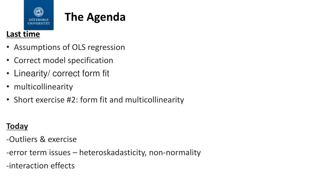
1. The Agenda Last time • Assumptions of OLS regression • Correctmodelspecification • Linearity/ correct form fit • multicollinearity • Short exercise #2: form fit and multicollinearity Today -Outliers & exercise -error term issues – heteroskadasticity, non-normality -interactioneffects

2. Exercise #2: checking for correct functional form and multicollinearity (practice1data.dta) *we want to explain variation in the share of women in parliament (DV) across countries as a function of corruption, population, and spending on primary education (IV’s) ***See Exercise 2 in GUL***

3. 1. Look at the variables – describe, sum, histogram

4. Histogram – hist yvar

5. 2. Bivariate correlations

6. 2. Bivariate correlations

7. 2. Bivariate correlations

8. 2. Bivariate correlations

9. 3. Multivariate regression 4. Interpretation - Effect of: • 1. education? • 2. corruption? • 3. population? • 4. constant? • 5. model F-stat? • 6. R2? • 7. MSE?

10. 5. Test model fit – near sig. ovtest…

11. 6. Adjustvariablesifneeded • Herewecan at least try toseeif the log transformation of the population fits the modelbetter gen log_pop = log( une_pop) pwcorripu_l_swlog_pop | ipu_l_swlog_pop -------------+------------------ ipu_l_sw | 1.0000 log_pop | 0.0168 1.0000

12. 7. Re-runwith transformed variable • Our previous R2 was 0.15 • Ourprevious MSE was 10.58 • Ourprevious p-value for the ovtestwas 0.12 • Q: Interpert the Log_popvariable? • A: a 1% change in population is assocaitedwith an increase in women by0.75*. (yeteffect non-significant…)

13. 8. Check multicollinearity • What do wethinkabouttheseresults? • Final interpretations?

14. OLS is fantastic if our data meets several assumptions, and before we make any inferences, we should always check: In order to make inference: Correct model specification - the linear model is suitable Error term is not correlated with X’s, ‘exogeneity’, E(εi|X1i,X2i,…, XNi,)=0 No severe multicollinearity The conditional standard deviation is the same for all levels of X (homoskedasticity) Error terms are normally distributed for all levels of X There are no severe outliers There is no autocorrelation The sample is selected randomly & is representative of the population Assumptions of OLS

15. 3. No extreme outliers • What do wemean by ’outliers’? • Outliersifundetected, canhave a severeimpacton yourβestimates. You must check for these, especiallywhereY’s or X’sarecontinuous. Survey data with all ordinalvariables less of a problem… Three waysweshouldthinkaboutoutlying observations: • Leverageoutlier– an observation far from the meanof Y or X (for ex., 2 or 3+ st. deviations from mean) • Residualoutlier– an observation that ’goes againstourprediction’ (e.g. has a lotoferror) • Influence: ifwetakethis observation out, do the resultschangesignficantly? A leverage outlier is not necessarily a problem (if it is in linewithourpredictions). However, a leverage outlier makes thingsverymisleadingif it is also a bigresidualoutlier, meaning it will be an influence observation.

17. use”crimedata.dta" • Explainingcrime rates in US stateswith3 IV’s • %metro area, • poverty rate % • %ofsingleparenthouseholds

18. use”crimedata.dta" • Run a regression explainingcrime in a state (# ofviolentcrimes/100,000 people): 3 IV’s • %metro area, • poverty rate % • %ofsingleparenthouseholds • Interpretation?

19. Detectionofinfluenceof obs: lvr2plot • A simple leverage residualplotcangiveus a clearvisual lvr2plot • We do thispost-regression in STATA • Y-axis = leverage • x- axis_ residual • Anyneartop right corner canespecially -bias results!

20. outliers via ‘studentized’ residuals Wecan check with normal residuals, buttheyaredependent on theirscale, which make it hard tocompare different models. Studentized residuals are adjusted. They are re-calculated residuals whereby the regression line is re-calculated by taking out each observation one at a time. We then compare the first estimates (all obs) with the estimates removing each obs, for each obs. For obs where the line moves a lot, the obs has a larger studentized residual..

21. Normal (raw), vs. studentizedresiduals Normal – predict res, residStudentized – predict r, rstandard Z and Stud can be related To the Z-score where 95% of The resid. fall within ± 2 std.dev

22. Looking at obs on extremes of distribution • predict r, rstudent • Command ’hilo’ • Specifywith ’show(#) howmanyyouwanttosee (default =10) • Any obs -2 or +2 (esp. -3 or +3) should be furtherlooked at

23. Influence of each observation: Cook’s D • In STATA, afteranyregression: predict d, cooksd If Cook’s d = 0 for an obs, than the obs has no influence, the higher the d value, the greater the influence. It is calcualted via an F-test, testingwhetherXi=Xi(minus obs i) affects the RSS The ’ruleofthumb’ for observations withpossiblytroublesomeinfluence is d > 4/n To avoidadding observations withmissing data, specify: ifd>4/51

24. Compareoutlier’s stats on variableswithsample

25. Measuringinfluence for each IV: DFBETA • dfbeta is a stastisticofinfluenceof obs for each IV in the model • It tellsushowmanystandard errorsthe coefficient WOULD CHANGE ifweremoved the obs • Typedfbetaafter a regression • A new variable is generated for each IV • Ex. DC increases Beta of % singleparentby roughly3.13*se (or 3.13*15.5) compared to regwithout DC • Dependent on scaleof Y and X! • Caution for anydfbetanumberabove: = 0.28

26. Example: with and without DC

27. Whatto do aboutoutliers? First, it depends on whattype of ’outlier’ an observation is! no ”right” answerhere, just be awareofiftheyexsist and howmucheffecttheyhave on the estimates, BUT: • Check for data error! 2. Create an obs. dummy for the outliers gen outlier= 1 ifccode==x replaceoutlier=0 ifoutlier==. 3. *Takeout the obs & re-runmodel & seeifanydifferences, run ’lfit’ and compareR²stats.. Reportanydifferences… usually in an appendix of a paper &/or footnote 3. Try a new functional form (log, normalizevariables) 4. Do nothing, leavethemin - just be transparent about it 5. Useweightedobservations

28. Robust regression (rreg) Robust regression can be used in any situation in which you would use OLS Can also be helpful in dealing with outliers after we decide that have no compelling reason to exclude them from the analysis.  In normal OLS, all observations are weighted equally. The idea of robust regression is to weigh the observations differently based on how “well behaved” they are. Basically, it is a form of weighted and reweighted OLS (WLS)

29. Robust regression (rreg) Stata's rreg command implements a version of robust regression. It runs the OLS regression, gets the Cook's D for each observation. Obs. with small residuals gets higher weight (1>), any obs. with Cook's distance greater than 1 (sever influence) are dropped. Using the Stata defaults, robust regression is about 95% as efficient as OLS (Hamilton, 1991).  In short, the most influential points are dropped, and then cases with large absolute residuals are down-weighted. Looking at our example data on crime in US states…

30. ORGANISATIONSNAMN (ÄNDRA SIDHUVUD VIA FLIKEN INFOGA-SIDHUVUD/SIDFOT)

31. exercise on outliers Open ’practicedata1’ datasetagain, and we’ll do the same regression as in example 1 See ’Exercise 3’ wordfile

32. Regression & lvrplot

33. Studentizedresiduals (accuracy) & Cook’s d (influence) • Any -2/+2 or especially -3/+3 observations should be on ourwatch-list!

34. Dfbeta • calculate the • = = 11.1 • 2/11.1 = 0.18 • What do weseehere? • Ex. Cuba increases the β of education by 0.45 (se) = .45 *1.3 = .585, comparedtowhen Cuba is excluded • Sweden increases the βof corruption by .32(se) = .32*.05 = 0.016, comparedtowhensweden is excluded.

35. Adjustmentstooutliers • Robust regression drop leverage ifcook’s d >4/n

36. Adjustmentstooutliers • Dropresidualoutliers (e.g. those < -2 or >2 on the studentizeds.e.

37. Assumptionsthatareerror-term violations: -normality-homoskadasticity-autocorrelation-independenceof observations

38. 4. mean of error=0, are normally distributed for all levels of X Key issues: • There is a probability distribution of Y for each level of X. A ‘hard’ assumption is that this distribution is normal (bell shaped) • Given that µy is the mean value of Y, the standard form of the model is where  is a random variable with a normal distribution with mean 0 and standard deviation .

39. Normality distribution of error terms While violations against any of the three former assumptions (1 Model specification – linearity 2, No extreme observations 3, (No strong multicollinearity)) could potentially result in bias in the estimated coefficients. However, violations against the assumptions concerning the residuals(4) absence of autocorrelation 5) normally distributed residuals and 6) homoskadasticity) may not necessarily not affect the estimated coefficients but it may affect and reduce your ability to perform inference and hypothesis testing. But they can, so it’s always good to check! Since the residuals distribution is the foundation to perform significance tests for the coefficients - it's the distribution that underlies the calculation of t- and P-values. This is especially true for smaller data samples. Esp. in small samples we want the residuals to be (approx) normally distributed.

40. Always important to do – for several assumptions To examine whether the regression model is appropriate for the data being analyzed, we can check the residual plots. Later we can do more ‘advanced’ tests to see if we’ve violated some assumptions Residual plots: 1. histogram of the residuals 2. Scatterplot residuals against the fitted values (y-hat). 3. Scatterplot residuals against the independent variables (x). 4. Scatterplot residuals over time if the data are chronological (more later in time series analysis). Analysis of Residual

41. Plotting the residuals – ex • Use the academicperformance data, and regress academicperformance on the %of ESL learners, %of students withfreemeals, and averageeducation of parents • regress api00 mealsellemer • Thenpredict the residuals: • predictr, resid • Plot the desnityof the residualsagainst a normal bellcurve – howclosearetheymatched? • kdensity r, normal • A qnormplot (plots the quantiles of a variable against the quantiles of a normal distribution) • qnorm r

42. Densityplotqnormplot

43. More ’formal’ tests • Shapiro-Wilk W test for normality. Tests proximity of our residual distribution compared wit the normal bell curve. Ho: residuals are normally distributed swilk r

44. 5. Homoskadasticity • Homoskedasticity: The error has a constant variance around our regression line • The opposite of this is: • Heteroskedasticity: The variance of the error depends on the values of Xs.

45. Whatdoeshetereoskadasticity look like? • Plotting the residualsagainst X, weshould not variancearound a fittedline

46. consequences • If you find heteroscedasticity, like multicollinearity, this will effect the EFFICIENCY of the model. • The calculation of standard errors, and thus P-values will be uncertain, since differences in residuals dispersions is depending on the level of the variables. • The effect of X on Y might be very significant at some levels of X, and less so at others, which makes a total significance calculation impossible. • Heteroscedasticity does not necessarily result in biased parameter estimates but OLS is no longer BLUE. • Risk for Type I or Type II error will increase (what are these again??) • E.g. ‘false positive’ & ‘false negative’

47. Howto check for Heteroskadasticity • A visualplotof the residuals over the fittedvaluesof Y: rvfplot, yline(0) Herewe do not wanttoseeanypattern – just a randominsignificantscatteringofdots.. Use the ’academicperformance data’, and regress academicperformance (api100) on the %of ESL learniners (ell), %of students withfreemeals (meals), and averageeducationofparents (ave_ed)

48. rvfplot, yline(0) • What do weobserve? • Looks kind of random, buterror term seemstonarrow as fittedvalues get higher..

49. More ’formal’ tests 2. Breusch-Pagan / Cook-Weisberg test -RegressesSq. Errors on X’s *good at detectinglinearhetereoskadascticity, but not for non-linear forms. Ho: no heteroskadascticity 3. Cameron & Trivedi'sIM test -similar, butincludesalsosqauredX’s in regression Ho: no heteroskadascticity **bothare sensitive and willoften be signficantevenwithonlyslight hetero…

50. If wefindsomething, wemight check individualIV’s and residualplots, and look at correlationsofIV’s and error