Download
1 / 99
990 likes | 1k Views
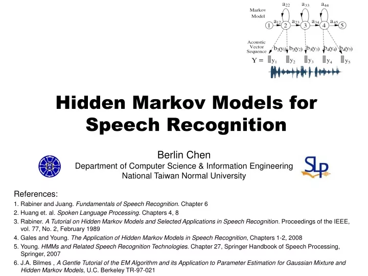
Hidden Markov Models for Speech Recognition. Berlin Chen Department of Computer Science & Information Engineering National Taiwan Normal University. References: 1. Rabiner and Juang. Fundamentals of Speech Recognition . Chapter 6

E N D
Hidden Markov Models for Speech Recognition Berlin Chen Department of Computer Science & Information Engineering National Taiwan Normal University References: 1. Rabiner and Juang. Fundamentals of Speech Recognition. Chapter 6 2. Huang et. al. Spoken Language Processing. Chapters 4, 8 3. Rabiner. A Tutorial on Hidden Markov Models and Selected Applications in Speech Recognition. Proceedings of the IEEE, vol. 77, No. 2, February 1989 4. Gales and Young. The Application of Hidden Markov Models in Speech Recognition, Chapters 1-2, 2008 5. Young. HMMs and Related Speech Recognition Technologies. Chapter 27, Springer Handbook of Speech Processing, Springer, 2007 6. J.A. Bilmes , A Gentle Tutorial of the EM Algorithm and its Application to Parameter Estimation for Gaussian Mixture and Hidden Markov Models, U.C. Berkeley TR-97-021
Hidden Markov Model (HMM):A Brief Overview History • Published in papers of Baum in late 1960s and early 1970s • Introduced to speech processing by Baker (CMU) and Jelinek (IBM) in the 1970s (discrete HMMs) • Then extended to continuous HMMs by Bell Labs Assumptions • Speech signal can be characterized as a parametric random (stochastic) process • Parameters can be estimated in a precise, well-defined manner Three fundamental problems • Evaluation of probability (likelihood) of a sequence of observations given a specific HMM • Adjustment of model parameters so as to best account for observed signals • Determination of a best sequence of model states
Stochastic Process • A stochastic process is a mathematical model of a probabilistic experiment that evolves in time and generate s a sequence of numeric values • Each numeric value in the sequence is modeled by a random variable • A stochastic process is just a (finite/infinite) sequence of random variables • Examples (a) The sequence of recorded values of a speech utterance (b) The sequence of daily prices of a stock (c) The sequence of hourly traffic loads at a node of a communication network (d) The sequence of radar measurements of the position of an airplane
Observable Markov Model • Observable Markov Model (Markov Chain) • First-order Markov chain of N states is a triple (S,A,) • S is a set of N states • A is the NN matrix of transition probabilities between statesP(st=j|st-1=i, st-2=k, ……)=P(st=j|st-1=i)Aij • is the vector of initial state probabilitiesj =P(s1=j) • The output of the process is the set of states at each instant of time, when each state corresponds to an observable event • The output in any given state is not random (deterministic!) • Too simple to describe the speech signal characteristics First-order and time-invariant assumptions
Observable Markov Model (cont.) First-order Markov chain of 2 states S1 S2 (Prev. State, Cur. State) S1 S2 S1 S1 Second-order Markov chain of 2 states S2S2 S2 S1
0.6 s1 A 0.3 0.3 0.1 0.1 0.2 0.5 0.7 s2 s3 0.2 C B Observable Markov Model (cont.) • Example 1: A 3-state Markov Chain State 1 generates symbol A only, State 2 generates symbol B only, and State 3 generates symbol C only • Given a sequence of observed symbols O={CABBCABC}, the only one corresponding state sequence is {S3S1S2S2S3S1S2S3}, and the corresponding probability is P(O|) =P(S3)P(S1|S3)P(S2|S1)P(S2|S2)P(S3|S2)P(S1|S3)P(S2|S1)P(S3|S2)=0.10.30.30.70.20.30.30.2=0.00002268
Observable Markov Model (cont.) • Example 2: A three-state Markov chain for the Dow Jones Industrial average The probability of 5 consecutive up days
Observable Markov Model (cont.) • Example 3: Given a Markov model, what is the mean occupancy duration of each state i Probability Time (Duration)
Hidden Markov Model (cont.) • HMM, an extended version of Observable Markov Model • The observation is turned to be a probabilistic function (discrete or continuous) of a state instead of an one-to-one correspondence of a state • The model is a doubly embedded stochastic process with an underlying stochastic process that is not directly observable (hidden) • What is hidden? The State Sequence!According to the observation sequence, we are not sure which state sequence generates it! • Elements of an HMM (the State-Output HMM) ={S,A,B,} • S is a set of N states • A is the NN matrix of transition probabilities between states • B is a set of N probability functions, each describing the observation probability with respect to a state • is the vector of initial state probabilities
Hidden Markov Model (cont.) • Two major assumptions • First order (Markov) assumption • The state transition depends only on the origin and destination • Time-invariant • Output-independent assumption • All observations are dependent on the state that generated them, not on neighboring observations
Hidden Markov Model (cont.) • Two major types of HMMs according to the observations • Discrete and finite observations: • The observations that all distinct states generate are finite in numberV={v1, v2, v3, ……, vM}, vkRL • In this case, the set of observation probability distributions B={bj(vk)}, is defined as bj(vk)=P(ot=vk|st=j), 1kM, 1jNot :observation at time t, st : state at time tfor state j, bj(vk) consists of only M probability values A left-to-right HMM
Hidden Markov Model (cont.) • Two major types of HMMs according to the observations • Continuous and infinite observations: • The observations that all distinct states generate are infinite and continuous, that is, V={v| vRd} • In this case, the set of observation probability distributions B={bj(v)}, is defined as bj(v)=fO|S(ot=v|st=j), 1jNbj(v) is a continuous probability density function (pdf)and is often a mixture of Multivariate Gaussian (Normal) Distributions Mean Vector Covariance Matrix Mixture Weight Observation Vector
Hidden Markov Model (cont.) • Multivariate Gaussian Distributions • When X=(X1, X2,…, Xd) is a d-dimensional random vector, the multivariate Gaussian pdf has the form: • If X1, X2,…, Xd are independent, the covariance matrix is reduced to diagonal covariance • The distribution as d independent scalar Gaussian distributions • Model complexity is significantly reduced
Hidden Markov Model (cont.) • Multivariate Gaussian Distributions
Hidden Markov Model (cont.) • Covariance matrix of the correlated feature vectors (Mel-frequency filter bank outputs) • Covariance matrix of the partially de-correlated feature vectors (MFCC without C0) • MFCC: Mel-frequency cepstral coefficients
Hidden Markov Model (cont.) • Multivariate Mixture Gaussian Distributions (cont.) • More complex distributions with multiple local maxima can be approximated by Gaussian (a unimodal distribution) mixture • Gaussian mixtures with enough mixture components can approximate any distribution
0.6 s1 {A:.3,B:.2,C:.5} 0.3 0.3 0.1 0.1 0.2 0.5 0.7 s2 s3 0.2 {A:.7,B:.1,C:.2} {A:.3,B:.6,C:.1} Hidden Markov Model (cont.) Ergodic HMM • Example 4: a 3-state discrete HMM • Given a sequence of observations O={ABC}, there are 27 possible corresponding state sequences, and therefore the corresponding probability is
Hidden Markov Model (cont.) • Notation : • O={o1o2o3……oT}: the observation (feature) sequence • S= {s1s2s3……sT} : the state sequence • : model, for HMM, ={A,B,} • P(O|) : 用model 計算 O的機率值 • P(O|S,) :在O是state sequence S所產生的前提下, 用model 計算 O的機率值 • P(O,S|) :用model 計算[O,S]兩者同時成立的機率值 • P(S|O,) : 在已知O的前提下, 用model 計算 S的機率值 • Useful formula • Bayesian Rule : chain rule
Hidden Markov Model (cont.) • Useful formula (Cont.): • Total Probability Theorem marginal probability B3 B2 B4 A B1 B5 Venn Diagram Expectation
Three Basic Problems for HMM • Given an observation sequence O=(o1,o2,…..,oT), and an HMM =(S,A,B,) • Problem 1:How to efficiently compute P(O|)? Evaluation problem • Problem 2:How to choose an optimal state sequence S=(s1,s2,……, sT)?Decoding Problem • Problem 3:How to adjust the model parameter =(A,B,)to maximizeP(O|)?Learning / Training Problem
Basic Problem 1 of HMM (cont.) Given O and , find P(O|)= Prob[observing O given ] • Direct Evaluation • Evaluating all possible state sequences of length T that generating observation sequence O • : The probability of each path S • By Markov assumption (First-order HMM) By chain rule By Markov assumption
Basic Problem 1 of HMM (cont.) • Direct Evaluation (cont.) • : The joint output probability along the path S • By output-independent assumption • The probability that a particular observation symbol/vector is emitted at time t depends only on the state st and is conditionally independent of the past observations By output-independent assumption
Basic Problem 1 of HMM (cont.) • Direct Evaluation (Cont.) • Huge Computation Requirements: O(NT) • Exponential computational complexity • A more efficient algorithms can be used to evaluate • Forward/Backward Procedure/Algorithm
s1 s3 s2 Basic Problem 1 of HMM (cont.) • Direct Evaluation (Cont.) State-time Trellis Diagram State s3 s3 s3 s3 s3 s2 s2 s2 s2 s2 s1 s1 s1 s1 s1 1 2 3 T-1 T Time O1 O2 O3 OT-1 OT si means bj(ot) has been computed aij means aij has been computed
Basic Problem 1 of HMM- The Forward Procedure • Base on the HMM assumptions, the calculation of and involves only , and , so it is possible to compute the likelihood with recursion on • Forward variable : • The probability that the HMM is in state i at time t having generating partial observation o1o2…ot
Basic Problem 1 of HMM- The Forward Procedure (cont.) • Algorithm • Complexity: O(N2T) • Based on the lattice (trellis) structure • Computed in a time-synchronous fashion from left-to-right, where each cell for time t is completely computed before proceeding to time t+1 • All state sequences, regardless how long previously, merge to N nodes (states) at each time instance t
Basic Problem 1 of HMM- The Forward Procedure (cont.) outputindependent assumption first-order Markov assumption
State s3 s3 s3 s3 s3 s1 s3 s2 s2 s2 s2 s2 s2 s1 s1 s1 s1 s1 1 2 3 T-1 T Time O1 O2 O3 OT-1 OT Basic Problem 1 of HMM- The Forward Procedure (cont.) • 3(3)=P(o1,o2,o3,s3=3|) =[2(1)*a13+ 2(2)*a23 +2(3)*a33]b3(o3) si means bj(ot) has been computed aij means aij has been computed
Basic Problem 1 of HMM- The Forward Procedure (cont.) • A three-state Hidden Markov Model for the Dow Jones Industrial average (0.6*0.35+0.5*0.02+0.4*0.009)*0.7 =0.1792 0.6 0.5 0.7 0.4 0.1 0.3
Basic Problem 1 of HMM- The Backward Procedure • Backward variable : t(i)=P(ot+1,ot+2,…..,oT|st=i , )
s1 s3 s3 s3 s2 s2 s2 s1 s3 Basic Problem 1 of HMM- The Backward Procedure (cont.) • 2(3)=P(o3,o4,…, oT|s2=3,) =a31* b1(o3)*3(1) +a32* b2(o3)*3(2)+a33* b1(o3)*3(3) State s3 s3 s3 s3 s2 s2 s2 s2 s1 s1 s1 s1 1 2 3 T-1 T Time O1 O2 O3 OT-1 OT
Basic Problem 2 of HMM How to choose an optimal state sequence S=(s1,s2,……, sT)? • The first optimal criterion: Choose the states st are individually most likely at each time t • Define a posteriori probability variable • Solution : st* = argi max [t(i)], 1 t T • Problem: maximizing the probability at each time t individually S*= s1*s2*…sT* may not be a valid sequence (e.g. ast*st+1* = 0) state occupation probability (count) – a soft alignment of HMM state to the observation (feature)
s1 s1 s3 s1 s3 s1 s2 s2 s2 s2 s2 s3 s2 s1 s3 s3 s3 s3 Basic Problem 2 of HMM (cont.) • P(s3 = 3 ,O |)=3(3)*3(3) 3(3) 3(3) State s3 s1 s1 s3 s3 a23=0 s2 s2 s2 s2 s2 s3 s3 s3 s3 s3 1 2 3 T-1 T time O1 O2 O3 OT-1 OT
Basic Problem 2 of HMM- The Viterbi Algorithm • The second optimal criterion:The Viterbi algorithm can be regarded as the dynamic programming algorithm applied to the HMM or as a modified forward algorithm • Instead of summing up probabilities from different paths coming to the same destination state, the Viterbi algorithm picks and remembers the best path • Find a single optimal state sequence S=(s1,s2,……, sT) • How to find the second, third, etc., optimal state sequences (difficult ?) • The Viterbi algorithm also can be illustrated in a trellis framework similar to the one for the forward algorithm • State-time trellis diagram
Basic Problem 2 of HMM- The Viterbi Algorithm (cont.) • Algorithm • Complexity: O(N2T)
s1 s3 s2 Basic Problem 2 of HMM- The Viterbi Algorithm (cont.) 3(3) State s3 s3 s3 s3 s3 s2 s2 s2 s2 s2 s1 s1 s1 s1 s1 1 2 3 T-1 T time O1 O2 O3 OT-1 OT
Basic Problem 2 of HMM- The Viterbi Algorithm (cont.) • A three-state Hidden Markov Model for the Dow Jones Industrial average 0.6 (0.6*0.35)*0.7 =0.147 0.5 0.7 0.4 0.1 0.3
Basic Problem 2 of HMM- The Viterbi Algorithm (cont.) • Algorithm in the logarithmic form
Homework-1 • A three-state Hidden Markov Model for the Dow Jones Industrial average • Find the probability: P(up, up, unchanged, down, unchanged, down, up|) • Fnd the optimal state sequence of the model which generates the observation sequence: (up, up, unchanged, down, unchanged, down, up)
Probability Addition in F-B Algorithm • In Forward-backward algorithm, operations usually implemented in logarithmic domain • Assume that we want to add and P1 P1+P2 logP1 logP2 log(P1+P2) P2 The values of can besaved in in a table to speedup the operations
Probability Addition in F-B Algorithm (cont.) • An example code #define LZERO (-1.0E10) // ~log(0) #define LSMALL (-0.5E10) // log values < LSMALL are set to LZERO #define minLogExp -log(-LZERO) // ~=-23 double LogAdd(double x, double y) { double temp,diff,z; if (x<y) { temp = x; x = y; y = temp; } diff = y-x; //notice that diff <= 0 if (diff<minLogExp) // if y’ is far smaller than x’ return (x<LSMALL) ? LZERO:x; else { z = exp(diff); return x+log(1.0+z); } }
Basic Problem 3 of HMMIntuitive View • How to adjust (re-estimate) the model parameter =(A,B,) to maximizeP(O1,…, OL|) or logP(O1,…, OL |)? • Belonging to a typical problem of “inferential statistics” • The most difficult of the three problems, because there is no known analytical method that maximizes the joint probability of the training data in a close form • The data is incomplete because of the hidden state sequences • Well-solved by the Baum-Welch (known as forward-backward) algorithm and EM (Expectation-Maximization) algorithm • Iterative update and improvement • Based on Maximum Likelihood (ML) criterion The “log of sum” form is difficult to deal with
Maximum Likelihood (ML) Estimation: A Schematic Depiction (1/2) • Hard Assignment • Given the data follow a multinomial distribution State S1 P(B| S1)=2/4=0.5 P(W| S1)=2/4=0.5
Maximum Likelihood (ML) Estimation: A Schematic Depiction (1/2) • Soft Assignment • Given the data follow a multinomial distribution • Maximize the likelihood of the data given the alignment State S1 State S2 0.7 0.3 0.4 0.6 P(B| S1)=(0.7+0.9)/ (0.7+0.4+0.9+0.5) =1.6/2.5=0.64 P(B| S2)=(0.3+0.1)/ (0.3+0.6+0.1+0.5) =0.4/1.5=0.27 0.9 0.1 P(W| S2)=( 0.6+0.5)/ (0.3+0.6+0.1+0.5) =0.11/1.5=0.73 0.5 0.5 P(W| S1)=(0.4+0.5)/ (0.7+0.4+0.9+0.5) =0.9/2.5=0.36
Basic Problem 3 of HMMIntuitive View (cont.) • Relationship between the forward and backward variables
Basic Problem 3 of HMMIntuitive View (cont.) j • Define a new variable: • Probability being at state i at time t and at state j at time t+1 • Recall the posteriori probability variable: i t+1 t
s3 s3 s1 s3 s1 s1 s1 s2 s2 s2 s2 s2 s2 s3 s2 s1 s3 s1 s1 s3 s1 Basic Problem 3 of HMMIntuitive View (cont.) • P(s3 = 3,s4 = 1,O |)=3(3)*a31*b1(o4)*1(4) State s3 s3 s3 s2 s2 s2 s1 s1 s1 1 2 3 4 T-1 T time O1 O2 O3 OT-1 OT
Basic Problem 3 of HMMIntuitive View (cont.) • A set of reasonable re-estimation formula for {A,} is Formulae for Single Training Utterance