State Variable Compensator Employing Full-State Feedback in Series with a Full State Observer

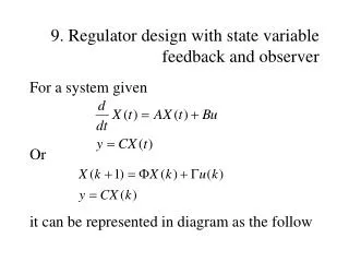
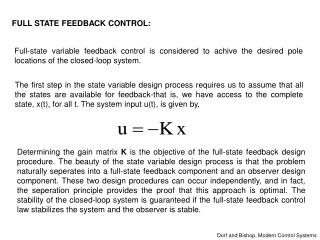
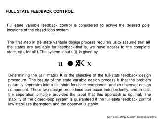
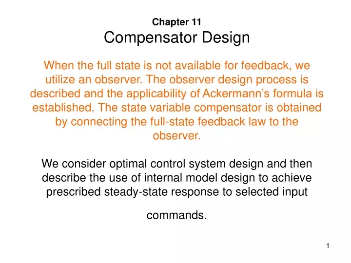
1. Chapter 11Compensator DesignWhen the full state is not available for feedback, we utilize an observer. The observer design process is described and the applicability of Ackermann’s formula is established. The state variable compensator is obtained by connecting the full-state feedback law to the observer.We consider optimal control system design and then describe the use of internal model design to achieve prescribed steady-state response to selected input commands.

2. x u y C System Model + Control Law -K Observer - C Compensator State Variable Compensator Employing Full-State Feedback in Series with a Full State Observer

3. Compensator DesignIntegrated Full-State Feedback and Observer Control Gain -K Observer Gain L u y + +

5. The goal is to verify that, with the value of u(t) we retain the stability of the closed-loop system and the observer. The characteristic equation associated with the previous equation is

6. The Performance of Feedback Control Systems • Because control systems are dynamics, their performance is usually specified in terms of both the transient response which is the response that disappears with time and the steady-state response which exists a long time following any input signal initiation. • Any physical system inherently suffers steady-state error in response to certain types of inputs. A system may have no steady-state error to a step input, but the same system may exhibit nonzero steady-state error to a ramp input. • Whether a given system will exhibit steady-state error for a given type of input depends on the type of open-loop transfer function of the system.

7. The System Performance • Modern control theory assumes that the systems engineer can specify quantitatively the required system performance. Then the performance index can be calculated or measured and used to evaluate the system’s performance. A quantitative measure of the performance of a system is necessary for the operation of modern adaptive control systems and the design of optimum systems. • Whether the aim is to improve the design of a system or to design a control system, a performance index must be chosen and measured. • A performance index is a quantitative measure of the performance of a system and is chosen so that emphasis is given to the important system specifications.

8. Optimal Control Systems • A system is considered an optimum control system when the system parameters are adjusted so that the index reaches an extreme value, commonly a minimum value. • A performance index, to be useful, must be a number that is always positive or zero. Then the best system is defined as the system that minimizes this index. • A suitable performance index is the integral of the square of the error, ISE. The time T is chosen so that the integral approaches a steady-state value. You may choose T as the settling time Ts

9. The Performance of a Control System in Terms of State Variables • The performance of a control system may be represented by integral performance measures [Section 5.9]. The design of a system must be based on minimizing a performance index such as the integral of the squared error (ISE). Systems that are adjusted to provide a minimum performance index are called optimal control systems. • The performance of a control system, written in terms of the state variables of a system, can be expressed in general as • Where x equals the state vector, u equals the control vector, and tf equals the final time. • We are interested in minimizing the error of the system; therefore when the desired state vector is represented as xd = 0, we are able to consider the error as identically equal to the value of the state vector. That is, we desire the system to be at equilibrium, x = xd= 0, and any deviation from equilibrium is considered an error.

10. Design of Optimal Systems using State Variable Feedback and Error-Squared Performance Indices: Consider the following control system in terms of x and u State variables Control signals x1 u1 Control System u2 x2 x3 um

11. Now Return to the Error-Squared Performance Index

12. To minimize the performance index J, we consider two equationsThe design steps are: first to determine the matrix P that satisfies the second equation when H is known. Second minimize J by determining the minimum of the first equation by adjusting one or more unspecified system parameters.

13. State Variable Feedback: State Variables x1 and x2 x2(0)/s x1(0)/s 1 1 1/s 1 1/s u x2 x1

15. 1/s 1/s x2 x1 R(s)=0 Y(s) U(s) - - k2 k1

16. Compensated Control System x2(0)/s x1(0)/s 1 1 1/s 1 1/s u x1 x2 -k2 = -2 -k1= -1

17. Design Example: Automatic Test SystemA automatic test system uses a DC motor to move a set of test probes as shown in Figure 11.23 in the textbook. The system uses a DC motor with an encoded disk to measure position and velocity. The parameters of the system are shown with K representing the required power amplifier. Amplifier Field Motor Vf u x2 x1 x3  K 1/s State variables x1 = ; x2 = d / dt; x3 = If

18. State Variable FeedbackThe goal is to select the gains so that the response to a step commandhas a settling time (with a 2%criterion) of less than 2 seconds andan overshoot of less than 4% Amplifier Field Motor + r x2 x1 x3 K  - 1/s k3 k2 k1

20. To achieve an accurate output position, we let k1 = 1 and determine k, k2 and k3. The aim is to find the characteristic equation

22. P11.1:

23. P11.3: An unstable robot system is described below by the vector differential equation. Design gain k so that the performance index is minimized.