Download
1 / 4
40 likes | 125 Views
Explore the concept of Gaussian mixture models and self-organizing maps to analyze data with multiple distributions and non-binary memberships. Learn to estimate posteriors, maximize parameters, and visualize results effectively.

E N D
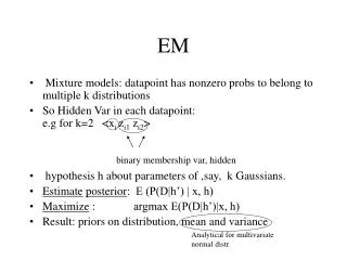
EM • Mixture models: datapoint has nonzero probs to belong to multiple k distributions • So Hidden Var in each datapoint: e.g for k=2 <xi zi1 zi2> • hypothesis h about parameters of ,say, k Gaussians. • Estimateposterior: E (P(D|h’) | x, h) • Maximize : argmax E(P(D|h’)|x, h) • Result: priors on distribution, mean and variance binary membership var, hidden Analytical for multivariate normal distr
VQ • vector quantization • map a set of M coding vectors (red) to a cloud of N data points (not shown) : Q(xi)=cj • ..using neighboring relations (Euclidian distance) • http://www.data-compression.com/vq.html
SOM • M “neurons”= M coding vectors (cfr. VQ) • But.. neurons are CONNECTED, so they form an “elastic net”. • Elasticity or mutual influence determined by a kernel function that is defined on a 2D grid • the coding vectors and their “projection (visualization)” on the 2D grid constitute the SOM
Useful Code • sDpima = som_read_data('d:\\patrick\\projects\\oefn_johan\\PIMADATAsorted2.txt'); • sDpima=som_normalize(sDpima, 'var') • sMap=som_make(…) • sMap=som_autolabel(sMap, sDpima, 'vote') • som_show(sMap,'norm','d') % basic visualization • som_show(sMap,'umat','all','empty','Labels') % UMatrix • som_show_add('label',sMap,'Textsize',8,'TextColor','r','Subplot',2) %labels • SORT DATASET (file) according to labels with e.g. spreadsheet program • % h1 = som_hits(sMap,sDpima.data(1:500,:)); -1’s • % h2 = som_hits(sMap,sDpima.data(501:768,:)); +1’s • % som_show_add('hit',[h1, h2],'MarkerColor',[1 0 0; 0 1 0],'Subplot',1)