Download
1 / 32
320 likes | 404 Views
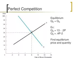
Perfect Competition. Chapter 12. Costs and Supply Decisions. How much should a firm supply? Firms and their managers should attempt to maximize profits (Profits = Revenues – Costs)

E N D
Perfect Competition Chapter 12
Costs and Supply Decisions • How much should a firm supply? • Firms and their managers should attempt to maximize profits (Profits = Revenues – Costs) • Select a pricing strategy that induces a demand for a product that generates highest revenue relative to the cost of production of that level of supply. • Profits depends on response of revenues to changes in production quantities.
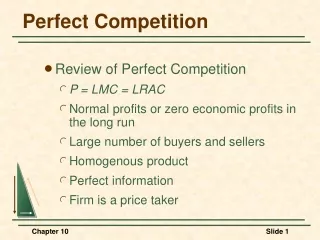
Perfect Competition/ Price Taking • We think of some markets as characterized by perfect competition • In competitive markets, no firm has the market power to set their own price. • Firms in perfectly competitive markets take their price as given. China Price Download
Non-differentiated goods • Large number of firms • All firms are small relative to the market • Free entry and exit. MES and Market Structure • If MES is relatively small in comparison with market demand: Many “small” firms in the market. $ Q
Revenues and Perfect Competition • Revenues = Price * Quantity • Average Revenue = Price • Marginal Revenue is the extra revenue generated by selling an extra good. • If production by a firm doesn’t shift the price, marginal revenue is the price.
Profit Maximization: Short Run • In the short-run, firm may only have a limited number of avenues along which they may vary production. • Cost of producing each good is likely to increase. But as long as the extra revenue that the good brings in exceeds the extra cost, it will be profitable to produce it. • Maximize profits by producing up to that point that price is equal to marginal cost. Beyond that, producing more goods only subtracts from profits.
Increase Production until marginal cost reaches the price level. MC P P ATC Q Q*
Revenues are price × quantity MC P P Revenues ATC Q Q*
Profits: Revenues - Costs MC P P Profits ATC Costs Q Q*
What if prices drop? MC P P Breakeven point ATC -Profits Costs P' Q Q**
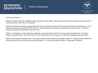
The average total cost of production (when marginal cost equals price) is above the new lower price. • If the firm sets production at a level such that price equals marginal cost, but that is the best they can do in the short run. • Firms only decision is to vary production costs along those dimensions that are available. • Should the firm shut down? • No. The firm has paid costs which cannot be retrieved [SUNK COSTS]. Since the firm cannot change this, they should ignore these sunk costs in making their marginal decision. • As long as prices exceeds variable costs, produce.
When should the firm stop production in the short-run? MC P Breakeven point ATC P P' AVC Dropout point Q Q**
Profit Maximization: Price is < 10 Dropout!
Adjustment in the Long Run • In the longer run, firms are able to adjust the size of their plant. (adjust the number of machines in the factory, adjust the number of oil rigs). • If profits are positive. Firms will seek to build new equipment as they compete for profits. • If profits are negative, firms will shut down equipment and sell it, or possibly go out of business. • Firms will adjust their physical plant until they are making profits again.
Final Exam • When 3 Feb 2013 (Sunday) 10:30-13:00. • Where L1: 3007 L2: 3008. • What: In class material, through here • How: The format of the exam will be similar to the midterm or the practice exams with a combination of multiple choice, short answer, calculation, and graphing questions. • Students should bring a calculator, writing instruments and an A4 sheet of paper with handwritten notes (must be handwritten, no Xerox or printout) on both sides.
Profit maximization and the supply curve • In the short-run, firms produce up to that point where price equal marginal cost. • Supply curve is the sum of the supply curves of the different firms in the market. • In the long-run, capacity will be adjusted to the point where profits are zero (i.e. where marginal cost equals average total cost). • Long run ATC curve is collection of points where MC = ATC and is the long-run supply curve.
Firm Level Supply Curve: Short Run P SFirm 1 SR ATC P* MC Output In the short run, MC curve is the relationship between firm price and production
Firm Level Supply Curve: Short Run P SFirm 2 SR ATC P* MC Output
Industry Level SupplyCurve:Short Run P +SFirm 2 +SFirm 3 SIndustry SFirm 1 Output In the short run, the sum of the MC curves is the relationship between price and industry production
Short Run Response to Increase in DemandIncrease Variable Inputs P D SIndustry 2 P** 1 P* D' Q* Q** Output
Firm Level Supply Curve: Short Run P SFirm 1 2 P** SR ATC 1 P* MC Output q* q** In the short run, MC curve is the relationship between firm price and production
Short-run profits attract new entrants P Profits SFirm 1 2 Profits P** SR ATC MC Output q* q** In the short run, MC curve is the relationship between firm price and production
New Entrants in the Long RunSupply Increases and Price Drops P D SIndustry +SFirm N+ 1 2 P** 3 P** 1 P* D' Q* Q** Q*** Output
Firm Level Response to New Entrants: Reduce Output P SFirm 1 2 P** SR ATC 3 P*** 1 P* MC Output q* q*** q** In the short run, MC curve is the relationship between firm price and production
New Entrants as Long as Profits at MESSupply Increases and Price Drops P +SFirm N+ 1 +SFirm N+ J D SIndustry 2 P** 3 P** 1 4 P* D' Q**** Q* Q** Q*** Output
Firm Level Response to New Entrants: Reduce Output P SFirm 1 2 P** SR ATC 3 P*** 1,4 P* MC Output q* q*** q** In the short run, MC curve is the relationship between firm price and production
Long Run, Supply is Flat along MES of New Entrants P +SIndustry D SIndustry 2 P** P** 1 4 SLR P* D' Q* Q** Q*** Q**** Output
Long Run Supply Curve • If all firms are exactly the same, then new firms have same MES as old firms and supply curve is flat. • In some cases, like oil drilling, new firms may have higher MES than old firms and supply curve is upward sloping. • Long run supply curve is flatter, more elastic than short-term supply curve.
Long Run Equilibrium • Firms are making zero profits. • Firms will be producing at their minimum efficient scale and at a minimum of ATC
Learning Outcomes Students should be able to • Characterize a perfectly competitive market. • Calculate total revenue, marginal revenue and profit for a firm in a competitive market. • Describe the supply curve in a competitive market in both the short and long run.