Download
1 / 64
640 likes | 768 Views
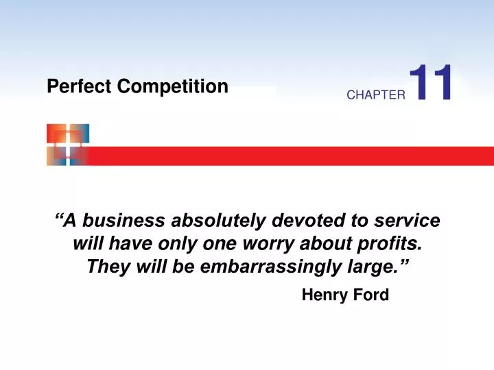
11. Perfect Competition. CHAPTER. “A business absolutely devoted to service will have only one worry about profits. They will be embarrassingly large.” Henry Ford. C H A P T E R C H E C K L I S T. When you have completed your study of this chapter, you will be able to.

E N D
11 Perfect Competition CHAPTER “A business absolutely devoted to service will have only one worry about profits. They will be embarrassingly large.” Henry Ford
C H A P T E R C H E C K L I S T • When you have completed your study of this chapter, you will be able to • 1Explain a perfectly competitive firm’s profit-maximizing choices and derive its supply curve. • 2 Explain how output, price, and profit are determined in the short run. 3 Explain how output, price, and profit are determined in the long run and explain why perfect competition is efficient.
MARKET TYPES • The four market types are • Perfect competition • Monopoly • Monopolistic competition • Oligopoly
MARKET TYPES • Perfect Competition - Characteristics • Many, many, many, many sellers, none so large that they can influence price. • Homogeneous product (buyers don’t care who they by from). • No barriers to entry or exit (easy to get in and out of market). • Long run economic profit = zero. (only earning normal profit) • Firms are price takers (no market power, so market sets same price for all firms).
11.1 A FIRM’S PROFIT-MAXIMIZING CHOICES • Revenue Concepts • In perfect competition, market demand and market supply determine price. • A firm’s total revenue equals the market price multiplied by the quantity sold. • A firm’s marginal revenue (MR) = change in total revenue (TR) that results from a one-unit increase in the quantity sold. • MR = Price
11.1 A FIRM’S PROFIT-MAXIMIZING CHOICES Part (a) shows the market for maple syrup. The market price is $8 a can.
11.1 A FIRM’S PROFIT-MAXIMIZING CHOICES In part (b), the market price determines the demand curve for the Dave’s syrup, which is also his marginal revenue curve.
11.1 A FIRM’S PROFIT-MAXIMIZING CHOICES In part (c), if Dave sells 10 cans of syrup a day, his total revenue is $80 a day at point A.
11.1 A FIRM’S PROFIT-MAXIMIZING CHOICES Dave’s total revenue curve is TR. The table shows the calculations of TR and MR.
11.1 A FIRM’S PROFIT-MAXIMIZING CHOICES • Profit-Maximizing Output • As output increases, total revenue (TR) increases. • But total cost (TC) also increases. • Because of diminishing marginal returns, TC eventually increases faster than TR. • There is one output level (Q) that maximizes economic profit (profit max), and a perfectly competitive firm chooses this output level.
11.1 A FIRM’S PROFIT-MAXIMIZING CHOICES • One way (the hard way) to find the profit-maximizing output is to use a firm’s total revenue and total cost curves. • Profit is maximized at output level where TR exceeds TC by the largest amount.
11.1 A FIRM’S PROFIT-MAXIMIZING CHOICES Total revenue increases as the quantity increases —shown by the TR curve. Total cost increases as the quantity increases—shown by the TC curve. As the quantity increases, economic profit (TR– TC) increases, reaches a maximum, and then decreases.
11.1 A FIRM’S PROFIT-MAXIMIZING CHOICES At low output levels, the firm incurs an economic loss. When total revenue exceeds total cost, the firm earns an economic profit. Profit is maximized when the gap between total revenue and total cost is the largest, at 10 cans per day.
11.1 A FIRM’S PROFIT-MAXIMIZING CHOICES • Marginal Analysis and the Output Decision • Marginal analysis (the simple way to find profit max) compares marginal revenue, MR, with marginal cost, MC. • As output (Q) increases, MR is constant but MC increases. • (NOTE: Maximizing profit = minimizing losses)
11.1 A FIRM’S PROFIT-MAXIMIZING CHOICES • If MR > MC: • The additional revenue from selling one more unit > the additional cost incurred to produce it. • Should increase output to increase economic profit. • If MR < MC: • The additional revenue from selling one more unit < the additional cost incurred to produce it. • Should decrease output to increase economic profit. • If MR = MC: PROFIT MAX • The additional revenue from selling one more unit = the additional cost incurred to produce it. • Economic profit would decrease if output increases or decreases, so economic profit is maximized where MR=MC.
11.1 A FIRM’S PROFIT-MAXIMIZING CHOICES Figure 11.3 shows the profit-maximizing output. Marginal revenue is a constant $8 per can.
11.1 A FIRM’S PROFIT-MAXIMIZING CHOICES Figure 11.3 shows the profit-maximizing output. Marginal cost decreases at low outputs but then increases.
11.1 A FIRM’S PROFIT-MAXIMIZING CHOICES Figure 11.3 shows the profit-maximizing output. Profit is maximized when marginal revenue equals marginal cost at 10 cans a day.
11.1 A FIRM’S PROFIT-MAXIMIZING CHOICES Figure 11.3 shows the profit-maximizing output. If output increases from 9 to 10 cans a day, MC=$7, which is less than MR=$8, and profit increases.
11.1 A FIRM’S PROFIT-MAXIMIZING CHOICES Figure 11.3 shows the profit-maximizing output. If output increases from 10 to 11 cans a day, MC=$9, which exceeds MR=$8, and profit decreases.
11.1 A FIRM’S PROFIT-MAXIMIZING CHOICES • Temporary Shutdown Decisions • If a firm is incurring an economic loss that it believes is temporary, it will remain in the market, and it might produce some output or temporarily shut down.
11.1 A FIRM’S PROFIT-MAXIMIZING CHOICES • If the firm shuts down temporarily, it incurs an economic loss equal to TFC. • If the firm produces some output, it incurs an economic loss equal to TFC plusTVC minusTR. • If TR > TVC, the firm’s economic loss is less than TFC. So it pays the firm to produce and incur an economic loss (it is covering at least SOME of their fixed costs, so they are better off than if they produced zero and had to pay all fixed costs out of pocket).
11.1 A FIRM’S PROFIT-MAXIMIZING CHOICES • If TR < TVC, the firm’s economic loss would exceed TFC. So the firm would shut down temporarily. • Loss = TFC when P = AVC. • So the firm produces some output if P>AVC and shuts down temporarily if P< AVC. • The firm’s shutdown point is where P=min AVC.
11.1 A FIRM’S PROFIT-MAXIMIZING CHOICES Marginal revenue curve is MR. The firm’s cost curves are MC, ATC, andAVC.
11.1 A FIRM’S PROFIT-MAXIMIZING CHOICES With a market price (and MR) of $3 a can, the firm minimizes its loss by producing 7 cans a day—at its shutdown point.
11.1 A FIRM’S PROFIT-MAXIMIZING CHOICES At the shutdown point, the firm incurs an economic loss equal to total fixed cost (TFC). (covering TVC, but none of fixed)
11.1 A FIRM’S PROFIT-MAXIMIZING CHOICES • The Firm’s Short-Run Supply Curve • A perfectly competitive firm’s short-run supply curve shows how the firm’s profit-maximizing output varies as the price varies, other things remaining the same. • Since a firm shuts down when P falls below AVC, the firm supply curve is the portion of the MC curve that lies above AVC.
11.2 OUTPUT, PRICE, PROFIT IN THE SHORT RUN • Market Supply in the Short Run • The market supply curve in the short run shows the quantity supplied at each price by a fixed number of firms. • The quantity supplied at a given price is the sum of the quantities supplied by all firms at that price.
11.2 OUTPUT, PRICE, PROFIT IN THE SHORT RUN Figure 11.6 shows the market supply curve in a market with 10,000 identical firms. At the shutdown price of $3, each firm produces either 0 or 7 cans a day.
11.2 OUTPUT, PRICE, PROFIT IN THE SHORT RUN At prices below the shutdown price, firms produce no output. At prices above the shutdown price, firms produce along their marginal cost curve.
11.2 OUTPUT, PRICE, PROFIT IN THE SHORT RUN At prices below the shutdown price, the market supply curve runs along the y-axis. At the shutdown price, the market supply is perfectly elastic. Above the shutdown price, the market supply slopes upward.
11.2 OUTPUT, PRICE, PROFIT IN THE SHORT RUN • Short-Run Equilibrium in Normal Times • Market demand and market supply determine the market price and quantity bought and sold. • Figure 11.7 on the next slide illustrates short-run equilibrium when the firm makes zero economic profit.
11.2 OUTPUT, PRICE, PROFIT IN THE SHORT RUN • Short-Run Equilibrium in Normal Times • NOTE: Profit per unit = P – ATC • Profit = (P – ATC) x Q • So, if P > ATC, firm earns positive economic profit. • if P < ATC, firm earns negative economic profit (loss) • if P = ATC, firm earns zero economic profit
11.2 OUTPUT, PRICE, PROFIT IN THE SHORT RUN In part (a), with market supply curve, S, and market demand curve, D1, the market price is $5 a can.
11.2 OUTPUT, PRICE, PROFIT IN THE SHORT RUN In part (b), marginal revenue is $5 a can. Dave produces 9 cans a day, where marginal cost equals marginal revenue.
11.2 OUTPUT, PRICE, PROFIT IN THE SHORT RUN At this quantity, price equals average total cost, so Dave makes zero economic profit.
11.2 OUTPUT, PRICE, PROFIT IN THE SHORT RUN • Short-Run Equilibrium in Good Times • In the short-run equilibrium that we’ve just examined, Dave made zero economic profit. • Although such an outcome is normal, economic profit can be positive or negative in the short run. • Figure 11.8 on the next slide illustrates short-run equilibrium when the firm makes a positive economic profit.
11.2 OUTPUT, PRICE, PROFIT IN THE SHORT RUN In part (a), with market demand curve D2 and market supply curve S, the market price is $8 a can.
11.2 OUTPUT, PRICE, PROFIT IN THE SHORT RUN In part (b), Dave’s marginal revenue is $8 a can. Dave produces 10 cans a day, where marginal cost equals marginal revenue.
11.2 OUTPUT, PRICE, PROFIT IN THE SHORT RUN At this quantity, price ($8 a can) exceeds average total cost ($5.10 a can). Dave makes an economic profit shown by the blue rectangle.
11.2 OUTPUT, PRICE, PROFIT IN THE SHORT RUN • Short-Run Equilibrium in Bad Times • In the short-run equilibrium that we’ve just examined, Dave is enjoying an economic profit. • But such an outcome is not inevitable. • Figure 11.9 on the next slide illustrates short-run equilibrium when the firm incurs an economic loss.
11.2 OUTPUT, PRICE, PROFIT IN THE SHORT RUN In part (a), with the market supply curve, S, andthe marketmarket demand curve, D3, the market price is $3 a can.
11.2 OUTPUT, PRICE, PROFIT IN THE SHORT RUN In part (b), Dave’s marginal revenue is $3 a can. Dave produces 7 cans a day, where marginal cost equals marginal revenue and not less than average variable cost.
11.2 OUTPUT, PRICE, PROFIT IN THE SHORT RUN At this quantity, price ($3 a can) is less than average total cost ($5.14 a can). Dave incurs an economic loss shown by the red rectangle.
11.3 OUTPUT, PRICE, PROFIT IN THE LONG RUN • Neither good times nor bad times last forever in perfect competition. • In the long run, a firm in perfect competition makes zero profit. • Figure 11.10 on the next slide illustrates equilibrium in the long run.
11.3 OUTPUT, PRICE, PROFIT IN THE LONG RUN Part (a) illustrates the firm in long-run equilibrium. The market price is $5 a can and Dave produces 9 cans a day.
11.3 OUTPUT, PRICE, PROFIT IN THE LONG RUN In part (a), minimum ATC is $5 a can. In the long run, Dave produces at minimum average total cost.
11.3 OUTPUT, PRICE, PROFIT IN THE LONG RUN If the price rises above or falls below $5 a can, market forces (entry and exit) move the price back to $5 a can.
11.3 OUTPUT, PRICE, PROFIT IN THE LONG RUN In the long-run, the price is pulled to $5 a can and Dave makes zero economic profit.