Download
1 / 16
240 likes | 1.69k Views
Hypothesis Testing in the Linear Regression Model. Based on Greene’s Note 8 . Classical Hypothesis Testing.

E N D
Hypothesis Testing in the Linear Regression Model Based on Greene’s Note 8
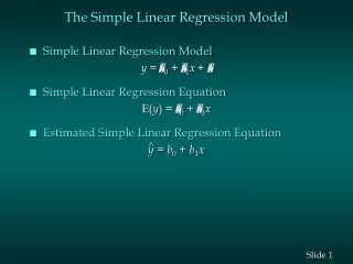
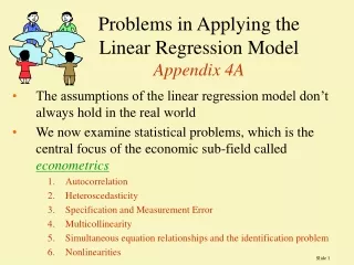
Classical Hypothesis Testing We are interested in using the linear regression to establish or cast doubt on the validity of a theory about the real world counterpart to our statistical model. The model is used to test hypotheses about the underlying data generating process.
Inference in the Linear Model Hypothesis testing: Formulating hypotheses: linear restrictions as a general framework Substantive restrictions: What is a "testable hypothesis?" Nested vs. nonnested models Methodological issues Classical (likelihood based approach): Are the data consistent with the hypothesis? Bayesian approach: How do the data affect our prior odds? The posterior odds ratio.
Testing a Hypothesis About a Parameter: Confidence Interval bk = the point estimate Std.Dev[bk] = sqr{[σ2(X’X)-1]kk} = vk Assume normality of ε for now: • bk ~ N[βk,vk2] for the true βk. • (bk-βk)/vk ~ N[0,1] Consider a range of plausible values of βk given the point estimate bk. bk +/- sampling error. • Measured in standard error units, • |(bk – βk)/vk| < z* • Larger z* greater probability (“confidence”) • Given normality, e.g., z* = 1.96 95%, z*=1.64590% • Plausible range for βk then is bk ± z* vk
Estimating the Confidence Interval Assume normality of ε for now: • bk ~ N[βk,vk2] for the true βk. • (bk-βk)/vk ~ N[0,1] vk = [σ2(X’X)-1]kk is not known because σ2 must be estimated. Using s2 instead of σ2, (bk-βk)/est.(vk) ~ t[n-K]. (Proof: ratio of normal to sqr(chi-squared)/df is pursued in your text.) Use critical values from t distribution instead of standard normal.
Testing a Hypothesis using a Confidence Interval Given the range of plausible values The confidence interval approach. Testing the hypothesis that a coefficient equals zero or some other particular value: Is the hypothesized value in the confidence interval? Is the hypothesized value within the range of plausible values
Wald Distance Measure Testing more generally about a single parameter. Sample estimate is bk Hypothesized value is βk How far is βk from bk? If too far, the hypothesis is inconsistent with the sample evidence. Measure distance in standard error units t = (bk - βk)/Estimated vk. If t is “large” (larger than critical value), reject the hypothesis.
Robust Tests • The Wald test generally will (when properly constructed) be more robust to failures of the narrow model assumptions than the t or F • Reason: Based on “robust” variance estimators and asymptotic results that hold in a wide range of circumstances. • Analysis: Later in the course – after developing asymptotics.
The General Linear Hypothesis: H0:R - q = 0 A unifying departure point: Regardless of the hypothesis, least squares is unbiased. Two approaches (1) Is Rb - q close to 0? Basing the test on the discrepancy vector: m = Rb - q. Using the Wald criterion: m(Var[m])-1m has a chi-squared distribution with J degrees of freedom But, Var[m] = R[2(X’X)-1]R. If we use our estimate of 2, we get an F[J,n-K], instead. (Note, this is based on using ee/(n-K) to estimate 2.) (2) We know that imposing the restrictions leads to a loss of fit. R2 must go down. Does it go down “a lot?” (I.e., significantly?). R2 = unrestricted model, R*2 = restricted model fit. F = { (R2 - R*2)/J } / [(1 - R2)/(n-K)] = F[J,n-K]. These are the same in the linear model
t and F statistics An important relationship between t and F For a single restriction, m = r’b - q. The variance is r’(Var[b])r The distance measure is m / standard error of m. The t-ratio is the square root of the F ratio.
Lagrange Multiplier Statistics Specific to the classical model: Recall the Lagrange multipliers: = [R(XX)-1R]-1m. Suppose we just test H0: = 0, using the Wald criterion. The resulting test statistic is just JF where F is the F statistic above. This is to be taken as a chi-squared statistic. (Note, again, using ee/(n-K) to estimate 2. If ee/n, instead, the more formal, likelihood based statistic results.)
Example Time series regression, LogG = 1 + 2logY + 3logPG + 4logPNC + 5logPUC + 6Year + Period = 1953 - 2004. A significant event occurs in October 1973. We will be interested to know if the model 1953 to 1973 is the same as from 1974 to 2004. Note that all coefficients in the model are elasticities.
Example • Simple Hypothesis: • Test about one ParameterH0 : 5 = 0 • Joint Hypotheses: • H0 : 4 = 5 = 0Using the Wald Statistic • Chow Test: Test for Structure Break • Structural break at the end of 1973 • J Test
J Test • Two Competitors • Model X:LogG = 1 + 2logY + 3logPG + 4logPNC + 5logPUC + 6Year + • Model Z:LogG = 1 + 2logY + 3logPG + 4logPN + 5logPD + 6PS + 7Year + • Note, each has its own set of regressors. Can't obtain either as a restriction on the other. • Strategy: See if the fitted values from the alternative model have any explanatory power in the null model. If so, reject the null.