Download
1 / 36
360 likes | 461 Views
Dynamic Origin-Destination Demand Flow Estimation under Congested Traffic Conditions. Xuesong Zhou (Univ. of Utah) Chung-Cheng Lu ( National Taipei University of Technology ) Kuilin Zhang ( Argonne National Lab ) Presented at INFORMS 2011 Annual Meeting. Motivation.

E N D
Dynamic Origin-Destination Demand Flow Estimation under Congested Traffic Conditions Xuesong Zhou (Univ. of Utah) Chung-Cheng Lu (National Taipei University of Technology) Kuilin Zhang (Argonne National Lab) Presented at INFORMS 2011 Annual Meeting
Motivation Why existing dynamic OD estimation methods are difficult to produce desirable results under congested conditions, when using link-flow proportions. 3 Difficulties in the past our new methods: 1. Partial derivatives with respect to path flow perturbation 2. Single-level path flow estimation framework with gap function term
Literature Review • Bi-level framework • Yang et al. (1992); Florianand Chen (1995) • Solution algorithm • Iterative estimation-assignment (IEA) algorithms • Sensitivity-analysis based algorithms (SAB)
Iterative Estimation-Assignment Method Dynamic OD Demand Estimation Flow Pattern Dynamic OD Demand Link Proportions Dynamic Traffic Assignment • Upper level Constrained ordinary least-squares problem s.t. non-negativity constraints Lower level: • Link flow proportion = Dynamic traffic assignment ( )) • Solution procedure • Measurement Equationscl,t=Σi,j,tp(l,t)(i,j,t)× di,j,t+
Difficulty in IEA Algorithms Upper-level optimization model does not consider the dependence of link-flow proportions on the OD flows. = function(d)
Sensitivity-Analysis Based (SAB) Algorithms • Approximate the derivatives through simulation • for each OD pair and each time interval in every iteration (Tavana, 2001) • Gradient approximation methods • Simultaneous Perturbation Stochastic Approximation (SPSA) framework by Balakrishnaet al. (2008); Ciprianiet al. (2011) • Difficulty: Computationally Intensive • Does not simultaneously achieve user equilibrium and minimize measurement deviations
Difficulty 3: How to Utilize Density/Travel Time Measurements Semi-continuous path trajectory Continuous path trajectory Point Point-to-point Loop Detector Automatic Vehicle Identification Automatic Vehicle Location Video Image Processing
Our Approach: Use Spatial Queue Model to evaluate partial derivatives with respect to path flow perturbation Inspired by study by Ghali and Smith (1995)
Case 1: Partially Congested Link Link inflow and outflow increase by 1 at two time stamps: entering time and end of queue duration, respectively.
Case 1: Partially Congested Link Link density (number of vehicles) increases by 1 between two timestamps: entering time, end of queue duration.
Case 1: Partially Congested Link The flows arriving between two time stamps experience the additional delay 1/c, because it takes 1/c to discharge this perturbation flow (similar to the results by Qian and Zhang 2011)
Case 2: Free-flow Conditions Number of vehicles (i.e., link density) increases by 1 from entering time to leaving time.
Case 2: Free-flow Conditions Link inflow and outflow increase by 1 at entering time and leaving time, respectively.
Case 2: Free-flow Conditions Individual travel times are not changed (= free flow travel time, FFTT)
Case 3: Two Partially Congested Links The perturbation flow on the second link starts at the end of queue duration of the first link; rather than the vehicle entering time on second link Here! Not Here! Similar work by Shen, Nie and Zhang (2007) for path marginal cost analysis
Case 4: Queue Spillback Individual extra delay depends on when the vehicle/perturbation flow joins in the queue.
Beyond A/D Curves: How to Model Queue Spillback? • Forward and backward wave representation in Newell’s simplified kinematic model
Our Method to Overcome for Difficulty 1 • Derive analytical, local gradients of different measurement types, with respect to flow perturbation • link flow, density and travel time • Valuable gradient information considers the dependences of link flow/density/travel time changes on OD flows
Now move to Challenge 2:Path flow Estimation Framework 1. Path flow adjustment Min (1) deviation between measured and estimated traffic states (2) the deviation between aggregated path flows and target OD flows S.T. dynamic user equilibrium (DUE) constraint 2. Aggregate path flows over all paths demand flows Demand flow target demand path flow target demand
Quick Review: Single-level OD Estimation • Linear programming PFE by Sherali et al. (1994) • Nonlinear programming PFE by Bell et al. (1997) on estimating stochastic UE path flows • Nie and Zhang (2008): single-level formulation based on variational inequalities • Qian and Zhang (2011) further incorporated the travel time gradients • Nie and Zhang (2010), and Shen and Wynter (2011) integrated the integral term in Beckmann’s UE formulation (1956) with the measurement deviations
Step 1: Lagrangian Reformulation • Describe the DUE constraint based on a gap function • DUE Gap • Dualize DUE constraint to the measurement deviation function with a non-negative (Lagrange) parameter • Measurement deviation function Z(r), including link flow, density, and travel time Minr, , L(r, , ) = z(r) + [g(r, ) ] g(r, ) = wp{r(w,,p)[c(w,,p)(w,)]}.
Step 2: Gradient Based Algorithm Adjust path flow on each path based on generalized gradient/Cost Individual gradients with respect to path flow adjustment Calculated based on the spatial queue model
Flowchart of the Algorithm Path flow adjustment based on all gradients
Our Contribution for Challenge 2 • New path flow-based optimization model for jointly solving the complex OD demand estimation and UE DTA problems • Simultaneous route and departure time user equilibrium (SRDUE) problem with elastic demand • Final solution is a set of path flow patterns satisfying “tolled user equilibrium” (Lawphongpanich and Hearn, 2004)
Numerical Experiment No.1 Congested two-link Corridor: Total capacity = 6000 vhc/hour Total demand = 8000 vhc/hour
Robustness of Our Algorithm under Different Input Conditions
Experiment 2 • A 2-mile section of I-210 Westbound, located in Los Angeles, CA
Observed Lane Volume vs. Estimated lane Volume on Entrance Link
Observed vs. Estimated Speed on Link from Off-ramp h to Station c
Preliminary Experiment: A Real-world Traffic Network 858 nodes 2,000 links 208 zones
Conclusions • Single-level, time-dependent OD demand estimation formulation, without using link proportions • A Lagrangian relaxation solution framework • Gradient-projection-based path flow adjustment process • Derive theoretically sound partial derivatives of link flow, density and travel time with respect to path flow perturbations
Historical OD demand Path flow decomposition Path flow vector 1 Path flow vector 2 Path flow vector 2 … Traffic Link Count Occupancy profile Speed profile Bluetooth records Measurement deviation based rapid gradient calculation generation Gradient-based path flow adjustment Gap function-based equilibration New path flow vectors Convergence detection Aggregated OD demand