Download
1 / 41
410 likes | 528 Views
ERROR RECOGNITION and IMAGE ANALYSIS. Ed Fomalont. PREAMBLE TO ERROR RECOGNITION and IMAGE ANALYSIS. Why are these two topics in the same lecture? Error recognition is used to determine defects in the data and image and to fix the problems.

E N D
ERROR RECOGNITION and IMAGE ANALYSIS Ed Fomalont
PREAMBLE TO ERROR RECOGNITION and IMAGE ANALYSIS • Why are these two topics in the same lecture? • Error recognition is used to determine defects in the data and image and to fix the problems. • Image analysis describes the almost infinite ways in which useful information and parameters can be extracted from the image. • Perhaps, these two topics are related by the reaction that one has when looking an image after ‘good’ calibration, editing, imaging, self-calibration. • If the reaction is Ninth Synthesis Imaging Summer School, Socorro, June 15-22, 2004
POSSIBLE IMAGE PROBLEMS Rats!! This can’t be right. This is either the most remarkable radio source ever, or I have made an error in making the image. Image rms, compared to the expected rms, is an important criterion. Ninth Synthesis Imaging Summer School, Socorro, June 15-22, 2004
HIGH QUALITY IMAGE Great!! After lots of work, I can finally analyze this image and get some interesting scientific results. (previous: 2 antennas with 10% error, 1 with 5 deg error and a few outlier points) Ninth Synthesis Imaging Summer School, Socorro, June 15-22, 2004
WHAT TO DO NEXT • So, the first serious display of an image leads one – • to inspect again and clean-up the data with repetition of some or all of the previous reduction steps. or • to image analysis and obtaining scientific results from the image. • But, first a digression on data and image display. Ninth Synthesis Imaging Summer School, Socorro, June 15-22, 2004
IMAGE DISPLAYS (1) The image is stored as numbers depicting the intensity of the emission in a rectangular-gridded array. (useful over slow links) Ninth Synthesis Imaging Summer School, Socorro, June 15-22, 2004
IMAGE DISPLAYS (2) Profile Plot Contour Plot These plots are easy to reproduce in printed documents Contour plots give good representation of faint emission. Profile plots give a good representation of the ‘mosque-like’ bright emission. Ninth Synthesis Imaging Summer School, Socorro, June 15-22, 2004
IMAGE DISPLAYS (3) Color Display Grey-scale Display Profile Plot Contour Plot TV-based displays are most useful and interactive: Grey-scale shows faint structure, but not good for high dynamic range. Color displays most flexible, especially for multiple images. Ninth Synthesis Imaging Summer School, Socorro, June 15-22, 2004
DATA DISPLAYS(1) List of u-v Data Ninth Synthesis Imaging Summer School, Socorro, June 15-22, 2004
DATA DISPLAYS(2) Visibility Amplitude versus Projected uv spacing General trend of data. Useful for relatively strong Sources. (Triple source model with large component in middle, see Non-imaging lecture) Ninth Synthesis Imaging Summer School, Socorro, June 15-22, 2004
DATA DISPLAYS(3) Plot of Visbility amplitude and Phase versus time for various baselines Good for determining the continuity of the data. should be relatively smooth with time Long baseline Short baseline Ninth Synthesis Imaging Summer School, Socorro, June 15-22, 2004
DATA DISPLAYS(4) Baselines Color Display of Visibility amplitude of each baseline with time. Usually interactive editing is possible. Example later. | | | T I M E | | | Ninth Synthesis Imaging Summer School, Socorro, June 15-22, 2004
USE IMAGE or UV-PLANE? Errors obey Fourier transform relations: Narrow features transform to wide features (vice-versa) Symmetries: amplitude errors symmetric features in image phase errors asymmetric features in image Orientations in (u-v) orthogonal orientation in image See Myers 2002 lecture for a graphical representation of (u-v) plane and sky transform pairs. Ninth Synthesis Imaging Summer School, Socorro, June 15-22, 2004
USE IMAGE or UV-PLANE? Errors easier to find if error feature is narrow: —Obvious outlier data (u-v) data points hardly affect image. 100 bad points in 100,000 data points is an 0.1% image error (unless the bad data points are 1 million Jy) USE DATA to find problem —Persistent small errors like a 5% antenna gain calibration are hard to see in (u-v) data (not an obvious outlier), but will produce a 1% effect in image with specific characteristics. USE IMAGE to find problem Ninth Synthesis Imaging Summer School, Socorro, June 15-22, 2004
ERROR RECOGNITION IN THE U-V PLANE Editing obvious errors in the u-v plane Mostly consistency checks assuming that the visibility cannot change much over a small change in u-v spacing. Also, double check gains and phases from calibration processes. These values should be relatively stable. See Summer school lecture notes in 2002 by Myers See ASP Vol 180, Ekers, Lecture 15, p321 Ninth Synthesis Imaging Summer School, Socorro, June 15-22, 2004
Editing using Visibility Amplitude versus uv spacing Nearly point source Lots of drop-outs Some lowish points Could remove all data less than 0.6 Jy, but Need more inform- ation. A baseline- time plot is better. Ninth Synthesis Imaging Summer School, Socorro, June 15-22, 2004
Editing using Time Series Plots Mostly occasional drop- outs. Hard to see, but drop outs and lower points at the beginning of each scan. (aips, aips++ task QUACK) Should apply same editing to all sources, even if too weak to see signal. Ninth Synthesis Imaging Summer School, Socorro, June 15-22, 2004
Editing noise-dominated Sources No source structure information available. All you can do is remove outlier points above 0.3 Jy. Precise level not important as long as large outliers removed. Other points consistent with noise. Ninth Synthesis Imaging Summer School, Socorro, June 15-22, 2004
RMS Phase with Time/Baseline Display Edit out scan in regions of high rms. Should edit Intervening data? Useful display for only one source at a time. Ninth Synthesis Imaging Summer School, Socorro, June 15-22, 2004
ERROR RECOGNITION IN THE IMAGE PLANE Editing from obvious errors in the image plane Any structure that looks ‘non-physical’, egs. stripes, rings, symmetric or anti-symmetric features. Build up experience from simple examples. Also lecture on high-dynamic range imaging, wide- field imaging have similar problems. Ninth Synthesis Imaging Summer School, Socorro, June 15-22, 2004
Example Error - 1 • Point source 2005+403 • process normally • self-cal, etc. • introduce errors • clean no errors: max 3.24 Jy rms 0.11 mJy 6-fold symmetric pattern due to VLA “Y” 13 scans over 12 hours 10% amp error all ant 1 time rms 2.0 mJy Also instrumental errors and real source variability Ninth Synthesis Imaging Summer School, Socorro, June 15-22, 2004
Example Error - 2 10 deg phase error 1 ant 1 time rms 0.49 mJy 20% amp error 1 ant 1 time rms 0.56 mJy anti-symmetric ridges symmetric ridges Ninth Synthesis Imaging Summer School, Socorro, June 15-22, 2004
Example Error – 3 (All from Myers 2002 lecture) 10 deg phase error 1 ant all times rms 2.0 mJy 20% amp error 1 ant all times rms 2.3 mJy rings – odd symmetry rings – even symmetry NOTE: 10 deg phase error equivalent to 20% amp error. That is why phase variations are generally more serious Ninth Synthesis Imaging Summer School, Socorro, June 15-22, 2004
DECONVOLUTION ERRORS • Even if data is perfect, image errors will occur because of poor deconvolution. • This is often the most serious problem associated with extended sources or those with limited (u-v) coverage • The problems can usually be recognized, if not always fixed. Get better (u-v) coverage! • Also, 3-D sky distortion, chromatic aberration and time-smearing distort the image (other lectures). Ninth Synthesis Imaging Summer School, Socorro, June 15-22, 2004
DIRTY IMAGE and BEAM (point spread function) Dirty Beam Dirty Image Source Model The dirty beam has large, complicated side-lobe structure (poor u-v coverage). It is hard to recognize the source in the dirty image. An extended source exaggerates the side-lobes. Ninth Synthesis Imaging Summer School, Socorro, June 15-22, 2004
CLEANING WINDOW SENSITIVITY Tight Box Middle Box Big Box Dirty Beam Small box around emission region Must know structure well to box this small. Reasonable box size for source Box whole area. Very dangerous with limited (u-v) coverage. Spurious emission is always associated with higher sidelobes in dirty-beam. Ninth Synthesis Imaging Summer School, Socorro, June 15-22, 2004
CLEAN INTERPOLATION PROBLEMS Measured (u-v) F.T. of Good image F.T. of Bad image Actual amplitude of sampled (u-v) points Clean effectively interpolated the sampled-data into the (u-v) plane. Clean was fooled by the orientation of the (u-v) coverage Both the good image and the bad image fit the data at the sampled points. But, the interpolation between points is different. Ninth Synthesis Imaging Summer School, Socorro, June 15-22, 2004
SUMMARY OF ERROR RECOGNITION Source structure should be ‘reasonable’, the rms image noise as expected, and the background featureless. If not, UV data Look for outliers in u-v data using several plotting methods. Check calibration gains and phases for instabilities. IMAGE plane Are defects related to possible data errors? Are defects related to possible deconvolution problems? Ninth Synthesis Imaging Summer School, Socorro, June 15-22, 2004
IMAGE ANALYSIS • Input: Well-calibrated Data-base and High Quality Image • Output: Parameterization and Interpretation of Image or a set of Images This is very open-ended Depends on source emission complexity Depends on the scientific goals Examples and ideas are given. Many software packages, besides AIPS and AIPS++ (eg. IDL) are available. Ninth Synthesis Imaging Summer School, Socorro, June 15-22, 2004
IMAGE ANALYSIS OUTLINE • Multi-Resolution of radio source. • Parameter Estimation of Discrete Components • Image Comparisons • Positional Information Ninth Synthesis Imaging Summer School, Socorro, June 15-22, 2004
IMAGE AT SEVERAL RESOLUTIONS Different aspects of source can be seen at the different resolutions, shown by the ellipse at the lower left. SAME DATA USED FOR ALL IMAGES For example, the outer components are very small. There is no extended emission beyond the three main components. Natural Uniform Low Ninth Synthesis Imaging Summer School, Socorro, June 15-22, 2004
PARAMETER ESTIMATION Parameters associated with discrete components • Fitting in the image • Assume source components are Gaussian-shaped • Deep cleaning restores image intensity with Gaussian-beam • True size * Beam size = Image size, if Gaussian-shaped. Hence, estimate of true size is relatively simple. • Fitting in (u-v) plane • Better estimates for small-diameter sources • Can fit to any source model (e.g. ring, disk) • Error estimates of parameters • Simple ad-hoc error estimates • Estimates from fitting programs Ninth Synthesis Imaging Summer School, Socorro, June 15-22, 2004
IMAGE FITTING AIPS task: JMFIT AIPS++ tool imagefitter Ninth Synthesis Imaging Summer School, Socorro, June 15-22, 2004
(U-V) DATA FITTING DIFMAP has best algorithm Fit model directly to (u-v) data Contour display of image Look at fit to model Ellipses show true size Ninth Synthesis Imaging Summer School, Socorro, June 15-22, 2004
COMPONENT ERROR ESTIMATES P = Component Peak Flux Density s = Image rms noise P/s = signal to noise = S B = Synthesized beam size W = Component image size DP = Peak error = s DX = Position error = B / 2S DW= Component image size error = B / 2S q = True component size = (W2– B2)1/2 Dq = Minimum component size = B / S1/2 Notice: Minimum component detectable size decreases only as S1/2. Ninth Synthesis Imaging Summer School, Socorro, June 15-22, 2004
IMAGE COMBINATION – LINEAR POLARIZATIONRecent work on Fornax-A I Q U Multi-purpose plot Contour – I Pol Grey scale – P Pol Line segments – P angle AIPS++ and AIPS have Many tools for polarization Analysis. Ninth Synthesis Imaging Summer School, Socorro, June 15-22, 2004
COMPARISON OF RADIO-X/RAY IMAGES Contours of radio intensity at 5 GHz of Fornax A with 6” resolution. Dots represent X-ray Intensity from four energies between 0.7 and 11.0 KeV from Chandra. Pixel separation is 0.5”. Color intensity represents X-ray intensity – convolution of above dots image to 6” Color represents hardness of X-ray (average frequency) Ninth Synthesis Imaging Summer School, Socorro, June 15-22, 2004
SPECTRAL LINE REPRESENTATIONS False color intensity Dim = Blue Bright = Red Integrated Mean Velocity Flux Velocity Dispersion (Spectral line lecture by Hibbard) Ninth Synthesis Imaging Summer School, Socorro, June 15-22, 2004
IMAGE REGISTRATION AND ACCURACY • Separation Accuracy of Components on One Image: Limited by signal to noise to limit of about 1% of resolution. Errors of 1:5000 for wide fields (20’ field 0.2” problems). • Images at Different Frequencies: Multi-frequency. Use same calibrator for all frequencies. Watch out at frequencies < 2 GHz when ionosphere can produce displacement. Minimize calibrator-target separation • Images at DifferentTimes (different configuration): Use same calibrator for all observations. Differences in position can occur up to 25% of resolution. Minimize calibrator-target separation. • Radio versus non-Radio Images: Header-information of non-radio images often much less accurate than that for radio. For accuracy <1”, often have to align using coincident objects. Ninth Synthesis Imaging Summer School, Socorro, June 15-22, 2004
DEEP RADIO / OPTICAL COMPARISON Finally, image analysis list from the sensitive VLA 1.4 GHz (5 mJy rms) and Subaru R and Z-band image (27-mag rms). 1. Register images to 0.15” accuracy. 2. Compile radio catalog of 900 sources, with relevant parameters. 3. Determine optical magnitudes and sizes. 4. Make radio/optical overlays for all objects. 5. Spectral index between 1.4 and 8.4 GHz VLA images. 6. Correlations of radio and optical properties, especially morphologies and displacements. Some of software in existing packages. Some has to be done adhoc. Ninth Synthesis Imaging Summer School, Socorro, June 15-22, 2004
SSA13 RADIO/OPTICAL FIELD Radio and optical alignment accurate to 0.15”. But, original optical registration about 0.5” with distortions of 1”. Optical field so crowded, need Good registration for reliable ID’s. Ninth Synthesis Imaging Summer School, Socorro, June 15-22, 2004