Modeling Cee Stud Compression: Elastic Buckling Loads

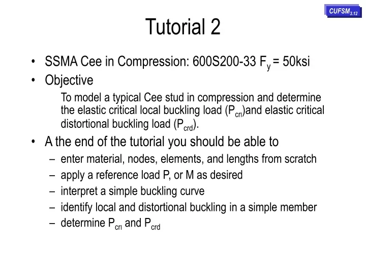
1. Tutorial 2 CUFSM3.12 • SSMA Cee in Compression: 600S200-33 Fy = 50ksi • Objective To model a typical Cee stud in compression and determine the elastic critical local buckling load (Pcrl)and elastic critical distortional buckling load (Pcrd). • A the end of the tutorial you should be able to • enter material, nodes, elements, and lengths from scratch • apply a reference load P, or M as desired • interpret a simple buckling curve • identify local and distortional buckling in a simple member • determine Pcrl and Pcrd

2. 2. SELECT 1. SELECT

3. This screen shows the default section that appears when you enter the Input screen for the first time. In our case we do not want to use this section so we need to start from scratch in order to enter our 600S200-33 member. Highlight each section: Material Properties, Nodes, Elements, Lengths and delete the current values.

4. Here we will enter in the material properties, in this case they will be for steel: E=29500 ksi, n=0.3 Here we need to enter in the node numbers and the coordinates that define the geometry. We just need to enter in the corner nodes (we will ignore the corner radii in this example). Here we enter in the elements. We need to give the connectivity of each element (what nodes are used to make the element) the thickness of each element and a number that refers back to the material being used. Finally we will need to enter in the half-wavelengths that we wish to do the analysis at.

5. Now enter in the material properties as shown to the left. Let’s define material #1. CUFSM allows you to define orthotropic materials, but in our case we are just using a simple isotropic material. Therefore Ex = Ey and nx = ny. For isotropic steel: E=29500 ksi, n=0.3, G=E/(2(1+n))=11346 ksi If our cross-section has multiple material types we could define a new material number and add a row to the material properties definition. That is not necessary in this case. Let’s start with the geometry next. Remember a 600S200-033 Cee section has:6 in. web2 in. flange0.62 in. lips0.0346 in. thickness

6. Now enter in the nodes and elements to define the bottom flange as shown to the left. Select Update Plot to see the results. The nodes include a node number, followed by the x and z coordinate followed by 4, “1’s” followed by 1.0. The 4 “1’s” indicate that there is no external longitudinal restraint at those nodes - for normal member analysis this is always the case. The final 50.0 is the stress input on that node, we use 50.0, but any value would do, because we are going to change this input later. **separate your entries by spaces** We are using simple outside dimensions, o.k. for this example. Lip = 0.62 in., flange = 2.00 in. lip bottom flange The element definition requires you to enter the element number, then its connectivity, then the element thickness, and finally the mat#, where 1 refers to the material we defined above. let’s finish the nodes and the elements…

7. Enter the last of the nodes and elements and select Update Plot. The model is nearly complete, but we need to consider a technical issue: how many elements do I need to get a good solution? Four elements in any “flat” in compression will provide a nicely converged answer. Even two elements does well, but 1 is too few. Press Double Elem. two times to increase the discretization of your member. Select Twice Note, use of the double elem. button is not reversible, (“no undo!”). You may want to save the model before doubling the elements.

8. After entering the lengths, select Properties to define the loading. Now we need to define the lengths. “Evenly” spacing the lengths in logspace as done below is a reasonable first estimate. For local buckling the half-wavelength of interest is close to the maximum dimension of the member (6 in. in this case). Distortional buckling is usually 2 to 8 times that length, and interest in the longer lengths depends on the application. let’s complete the loading. enter in lengths as shown Maximize the screen, if you can’t see the cursor.

9. Basic properties of the cross-section are shown above. The area, centroid, moments of inertia etc. should be what you expect, otherwise you may have made a mistake entering in the data.. relevant axes, origin, etc. are all shown on the cross-section. Bimoment for generating warping stress. An explicit example is given in overview. Finite strip analysis requires that you enter in a reference longitudinal stress. The buckling load factor output is a multiplier times this reference stress. The tools to the left make entering in the reference stress easier. For example,enter in 50 for fySelect calculate P and MUncheck PSelect Generate Stress Using checked P and M

10. Go back to the input page to see the result of generating stress using the “M” you checked. The loads are generated based on the fy you select. So, the generated P is the squash or yield load (Py) for this section. The M is the moment that causes first yield (My) etc. Based on the loads you check off, a stress distribution is generated. Note, for this symmetric section the maximum and minimum stresses are equal to the inputted fy.

11. Return to properties to remove this bending stress and define a compressive stress on the stud instead. Here we can see that the generated stress has placed a pure bending stress gradient on our member, note the entries in “Nodes” to the right and the values shown on the plot.

12. 1 select 1, analysis will proceed Now our reference load is Py, the squash load. So, if the buckling load factor is 0.5 then elastic critical buckling is at 0.5Py. You can load with any reference stresses that are convenient for your application. Maximum stress = 1.0, or fy are often convenient choices. Enter the yield stress, calculate the P and M values, and generate a pure compression stress.

13. change the half-wavelength to 5 and hit Plot Mode The local buckling mode is shown to the right. Note, that there is no translation at the folds, only rotation. The load factor is 0.10, so elastic critical local buckling (Pcrl) occurs at 0.10Py in this member. We do not have enough lengths! Go back to input, add more lengths between 10 and 30 and re-analyze (see Tutorial 1 for adding lengths)

14. Distortional buckling is identified at a half-wavelength of 26 in. The elastic critical distortional buckling load Pcrd=0.32Py change the half-wavelength to 26 and hit Plot Mode What exists at longer half-wavelengths, for example, 300 in.? Change the half-wavelength and select Plot Mode

15. What if? What happens if the member is thicker? Save these results as 600S200-033, change to a 600S200-097 with a t=0.1017 using the Input page, reanalyze and save the results as 600S200-097. Then use the compare button to look at the two analyses. At 300 in. the lowest buckling mode, is weak-axis flexural buckling of the column, as shown to the left.

16. The comparison post-processor allows you to examine up to 8 different runs at the same time. Useful when comparing different loading, geometry, or other changes. all key info. summarized here, in this case we are looking at local buckling of 600S200-033 note, the thickness difference in the elements when you change between File 2 an File 3. Remember the reference loads were equal to Py, but the Py of the two members are not the same because the area is not the same… Distortional Local

17. Tutorial 2: Conclusion CUFSM3.12 • SSMA Cee in Compression: 600S200-33 Fy = 50ksi • Objective To model a typical Cee stud in compression and determine the elastic critical local buckling load (Pcrl)and elastic critical distortional buckling load (Pcrd). • A the end of the tutorial you should be able to • enter material, nodes, elements, and lengths from scratch • apply a reference load P, or M as desired • interpret a simple buckling curve • identify local and distortional buckling in a simple member • determine Pcrl and Pcrd