NECSI Summer School 2008 Week 2: Complex Systems Modeling and Networks Network Models

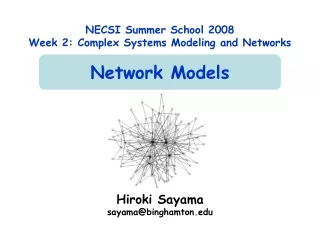
1. NECSI Summer School 2008Week 2: Complex Systems Modeling and NetworksNetwork Models Hiroki Sayama sayama@binghamton.edu

2. Models of complex systems • Cellular automata • Parts are connected in a regular grid • Agent-based models • Parts can move in a continuous space and interact based on physical proximity • Network models • Parts can be connected arbitrarily, not restricted by their spatial locations • Logical/social relationships among parts

3. Representation of Networks

4. Networks • Network (graph) = nodes (vertices) & links (edges) 1 Nodes = 1, 2, 3, 4, 5 Links = 1<->2, 1<->3, 1<->5, 2<->3, 2<->4, 2<->5, 3<->4, 3<->5, 4<->5 (Nodes may have states; links may have directions and weights) 3 2 4 5

5. Representation of a network • Adjacency matrix: A matrix with rows and columns labeled by nodes, where element aij shows the number of links going from node i to node j (becomes symmetric for undirected graph) • Adjacency list: A list of links whose element i->j shows a link going from node i to node j

6. 1 3 2 4 5 Exercise • Represent the following network in: • Adjacency matrix • Adjacency list

7. Measuring Topological Properties of Networks

8. Topological properties of networks • Number of nodes • Number of links • Average degree (# of links per node) • Number of connected components • Connectivity measures • Diameter • Clustering coefficient • Degree distribution

9. Diameter • In mathematics: Maximum of shortest path lengths between pairs of nodes • In recent network theory: Average shortest path lengths • Characterizes how large the world being modeled is • A small diameter implies that the network is well connected globally

10. Clustering coefficient • For each node: • Let n be the number of its neighbor nodes • Let m be the number of links among the k neighbors • Calculate c = m / (n choose 2) Then C = <c> (the average of c) • C indicates the average probability for two of one’s friends to be friends too • A large C implies that the network is well connected locally to form a cluster

11. Degree distribution P(k) = # of nodes with degree k • Gives a rough profile of how the connectivity is distributed within the network Sk P(k) = total number of nodes

12. Several Well-Known Network Models

13. Erdös-Rényi random network model • N nodes are provided from the beginning • For each of the N(N-1)/2 pairs of nodes, a link will be created independently with probability p

14. Exercise • Create and plot several ER random networks using NetworkX • Measure their properties • Study how the number of connected components and the diameter of random networks change with increasing link probability (for the same number of nodes, e.g. n=100)

15. Watts-Strogatz small-world network model • Nodes are initially arranged in a circle • Each node is connected to k nearest neighbors • Then edges are rewired randomly with probability p

16. Exercise • Create and plot several WS small-world networks using NetworkX • Measure their properties • Study how the diameter and the clustering coefficient of WS networks change with increasing rewiring probability (for the same number of nodes, e.g. n=100)

17. Barabási-Albert scale-free network model • Nodes are sequentially added to the network one by one • When adding a new node, it is connected to m nodes chosen from the existing network • Probability for a node to be chosen is proportional to its degree

18. Exercise • Plot degree distributions of several different networks described here (use large number of nodes, e.g. 10,000) • Compare their properties

19. Dynamics on Complex Networks

20. Dynamics on complex networks • Dynamical state changes considered on complex network topologies • Regulatory dynamics on gene/protein networks • Population dynamics on ecological networks • Disease infection on social networks • Information/culture propagation on organizational/social networks

21. Example: Epidemics on networks • Initially, a small fraction of nodes are infected by a disease • An infected node will recover and become susceptible with probability pr • If a susceptible node has an infected neighbor, it will be infected with probability pi (per infected neighbor) • Does the disease stay in the network?

22. Exercise • Study the effects of infection/ recovery probabilities on the fixation of a disease on a random social network • In what condition will the disease remain within society? • In what condition will it go away? • Is the transition smooth, or sharp?

23. Exercise • Do the same experiments with WS small-world networks and BA scale-free networks • Compare their properties