Download
1 / 34
340 likes | 351 Views
RESEARCH PRESENTATION :. An overview of work done so far in 2006. Madhulika Pannuri Intelligent Electronic Systems Human and Systems Engineering Center for Advanced Vehicular Systems. Abstract. ABSTRACT: Language Model ABNF:

E N D
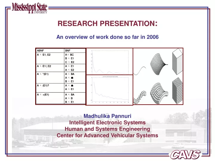
RESEARCH PRESENTATION: An overview of work done so far in 2006 Madhulika Pannuri Intelligent Electronic Systems Human and Systems Engineering Center for Advanced Vehicular Systems
Abstract • ABSTRACT: • Language Model ABNF: • The LanguageModel ABNF reads in a set of productions in the form of ABNF and converts them to BNF. These productions are passes to LanguageModel BNF in the form they are received. • Optimum time Delay estimation: • Computes optimum time delay for re-constructing phase space. Auto Mutual Information is used for finding optimum time delay. • Dimension Estimation: • The dimension of an attractor is a measure of its geometric scaling properties and is ‘the most basic property of an attractor’. Though there are many dimensions, we will be implementing ‘Correlation Dimension’ and ‘Lyapunov Dimension’.
Language Model ABNF • Why conversion from ABNF to BNF? • ABNF balances compactness and simplicity, with reasonable representational power. • Differences: The differences between BNF and ABNF involve naming rules, repetition, alternatives, order-independence and value ranges. • Removing the meta symbols makes it easy to convert it to finite state machines (IHD). • Problem: Converting any given ABNF to BNF is impossible. So, generalize the algorithm so that most of the expressions can be converted. • The steps for conversion involve removing meta symbols one after the other. There were complications like multiple nesting. • Ex: * (+(a, n) | (b | s))
Language Model ABNF • Concatenation: • Removing concatenation requires two new rules with new names to be introduced. The last two productions resulting from conversion are not valid CFG’s but shorter than the original. • Alternation: • The production is replaced with a pair of productions. They may or may not be legal CFG’s. • Kleene Star: • New variable is introduced and the production is replaced. Gives rise to epsilon transition. • Kleene Plus: • Similar to Kleene Plus. No null transition.
Optimum time delay estimation • Why calculating time delay ? • If we have a trajectory from a chaotic system and we only have data from one of the system variables, there's a neat theorem that says you can reconstruct a copy of the attractor of the system by lagging the time series to embed it in more dimensions. • In other words, if we have a point F( x, y, z, t) which is along some strange attractor, and we can only measure F(z,t), we can plot F (z, z + N, z + 2N, t), and the resulting object will be topologically identical to the original attractor ..!!! • Method of time delays provides a relatively simple way of constructing an attractor from single experimental time series. • So, how do we choose time delay ? • Choosing optimum time delay is not trivial as the dynamical properties of the reconstructed attractor are to be amenable for subsequent analysis. • For an infinite amount of noise free data, we are free to choose arbitrarily, the time delay.
Optimum time delay estimation • For smaller values of tau, s(t) and s(t+tau) are very close to each other in numerical value, and hence they are not independent of each other. • For large values of tau, s(t) and s(t+ tau) are completely independent of each other, and any connection between them in the case of chaotic attractor is random because of butterfly effect. • We need a criterion for intermediate choice that is large enough so that s(t) and s(t+tau) are independent but not so large that s(t) and s(t+tau) are completely independent in statistical sense. • Time delay is a multiple of sampling time (data is available at these times only). • There are four common methods for determining an optimum time delay: • Visual Inspection of reconstructed attractors: • The simplest way to choose tau. • Consider successively larger values of tau and then visually inspect the phase portrait of the resulting attractor. • Choosing the tau value which appears to give the most spread out attractor. • Disadvantage: • This produces reasonable results with relatively simple systems.
Methods to estimate optimum time delay • 2. Dominant period relationship: • We use the property that time delay is one quarter of the dominant period. • Advantage: • Quick and easy method for determining tau. • Disadvantages: • Can be used for low dimensional systems . • Many complex systems do not possess a single dominant frequency. • The Autocorrelation function: • The auto correlation function C, compares two data points in the time series separated by delay tau, and is defined as, • The delay for the attractor reconstruction, tau, is then taken at a specific threshold value of C. • The behavior of C is inconsistent .
Feature Extraction in Speech Recognition • 4.Minimum auto mutual Information method: • The Mutual Information is given by: • When the mutual information is minimum, the attractor is as spread out as much as possible. This condition for the choice of delay time is known as ‘minimum mutual information criterion’. • Practical Implementation: • To calculate the mutual information, the 2D reconstruction of an attractor is partitioned into a grid of Nc columns and Nr rows. • Discrete probability density functions for X(i) and X(i+tau) are generated by summing the data points in each row and column of the grid respectively and dividing by the total number of attractor points. • The joint probability of occurance P(k, l) of the attractor in any particular box is calculated by counting the number of discrete points in the box and dividing by the total number of points on the attractor trajectory. • The value of tau which gives the first minimum is the attractor reconstruction delay.
Doubly Stochastic Systems • The 1-coin model is observable because the output sequence can be mapped to a specific sequence of state transitions • The remaining models are hidden because the underlying state sequence cannot be directly inferred from the output sequence
Open-Loop Error Error Optimum Training Set Error Model Complexity • Machine Learning in Acoustic Modeling • Structural optimization often guided by an Occam’s Razor approach • Trading goodness of fit and model complexity • Examples: MDL, BIC, AIC, Structural Risk Minimization, Automatic Relevance Determination
Summary • What we haven’t talked about: duration models, adaptation, normalization, confidence measures, posterior-based scoring, hybrid systems, discriminative training, and much, much more… • Applications of these models to language (Hazen), dialog (Phillips, Seneff), machine translation (Vogel, Papineni), and other HLT applications • Machine learning approaches to human language technology are still in their infancy (Bilmes) • A mathematical framework for integration of knowledge and metadata will be critical in the next 10 years. • Information extraction in a multilingual environment -- a time of great opportunity!
Appendix: Relevant Publications • Useful textbooks: • X. Huang, A. Acero, and H.W. Hon, Spoken Language Processing - A Guide to Theory, Algorithm, and System Development, Prentice Hall, ISBN: 0-13-022616-5, 2001. • D. Jurafsky and J.H. Martin, SPEECH and LANGUAGE PROCESSING: An Introduction to Natural Language Processing, Computational Linguistics, and Speech Recognition, Prentice-Hall, ISBN: 0-13-095069-6, 2000. • F. Jelinek, Statistical Methods for Speech Recognition, MIT Press, ISBN: 0-262-10066-5, 1998. • L.R. Rabiner and B.W. Juang, Fundamentals of Speech Recognition, Prentice-Hall, ISBN: 0-13-015157-2, 1993. • J. Deller, et. al., Discrete-Time Processing of Speech Signals, MacMillan Publishing Co., ISBN: 0-7803-5386-2, 2000. • R.O. Duda, P.E. Hart, and D.G. Stork, Pattern Classification, Second Edition, Wiley Interscience, ISBN: 0-471-05669-3, 2000 (supporting material available at http://rii.ricoh.com/~stork/DHS.html). • D. MacKay, Information Theory, Inference, and Learning Algorithms, Cambridge University Press, 2003. • Relevant online resources: • “Intelligent Electronic Systems,” http://www.cavs.msstate.edu/hse/ies, Center for Advanced Vehicular Systems, Mississippi State University, Mississippi State, Mississippi, USA, June 2005. • Internet-Accessible Speech Recognition Technology,” http://www.cavs.msstate.edu/hse/ies/projects/speech, June 2005. • “Speech and Signal Processing Demonstrations,” http://www.cavs.msstate.edu/hse/ies/projects/speech/software/demonstrations, June 2005. • “Fundamentals of Speech Recognition,” http://www.isip.msstate.edu/publications/courses/ece_8463, September 2004.
Interactive Software: Java applets, GUIs, dialog systems, code generators, and more • Speech Recognition Toolkits: compare SVMs and RVMs to standard approaches using a state of the art ASR toolkit • Foundation Classes: generic C++ implementations of many popular statistical modeling approaches • Fun Stuff: have you seen our campus bus tracking system? Or our Home Shopping Channel commercial? • Appendix: Relevant Resources
Speech recognition • State of the art • Statistical (e.g., HMM) • Continuous speech • Large vocabulary • Speaker independent • Goal: Accelerate research • Flexibility, Extensibility, Modular • Efficient (C++, Parallel Proc.) • Easy to Use (documentation) • Toolkits, GUIs • Benefit: Technology • Standard benchmarks • Conversational speech • Appendix: Public Domain Speech Recognition Technology
Extensive online software documentation, tutorials, and training materials • Graduate courses and web-based instruction • Self-documenting software • Summer workshops at which students receive intensive hands-on training • Jointly develop advanced prototypes in partnerships with commercial entities • Appendix: IES Is More Than Just Software
“Though linear statistical models have dominated the literature for the past 100 years, they have yet to explain simple physical phenomena.” • Motivated by a phase-locked loop analogy • Application of principles of chaos and strange attractor theory to acoustic modeling in speech • Baseline comparisons to other nonlinear methods • Expected outcomes: • Reduced complexity of statistical models for speech (two order of magnitude reduction) • High performance channel-independent text-independent speaker verification/identification • Appendix: Nonlinear Statistical Modeling of Speech
Expert Systems Discriminative Methods Statistical Methods (Generative) Knowledge Integration Analog Systems Open Loop Analysis • Appendix: An Algorithm Retrospective of HLT • Observations: • Information theory preceded modern computing. • Early research focused on basic science. • Computing capacity has enabled engineering methods. • We are now “knowledge-challenged.”
Physical Sciences:Physics, Acoustics, Linguistics Engineering Sciences:EE, CPE, Human Factors Computing Sciences: Comp. Sci., Comp. Ling. Cognitive Sciences:Psychology, Neurophysiology • A Historical Perspective of Prominent Disciplines • Observations: • Field continually accumulating new expertise. • As obvious mathematical techniques have been exhausted (“low-hanging fruit”), there will be a return to basic science (e.g., fMRI brain activity imaging).
A priori expert knowledge created a generation of highly constrained systems (e.g. isolated word recognition, parsing of written text, fixed-font OCR). Performance • Statistical methods created a generation of data-driven approaches that supplanted expert systems (e.g., conversational speech to text, speech synthesis, machine translation from parallel text). … but that isn’t the end of the story … Source of Knowledge • Evolution of Knowledge and Intelligence in HLT Systems • A number of fundamental problem still remain (e.g., channel and noise robustness, less dense or less common languages). • The solution will require approaches that use expert knowledge from related, more dense domains (e.g., similar languages) and the ability to learn from small amounts of target data (e.g., autonomic).
Appendix: The Impact of Supercomputers on Research • Total available cycles for speech research from 1983 to 1993: 90 TeraMIPS • MS State Empire cluster (1,000 1 GHz processors):90 TeraMIPS per day • A Day in a Life: 24 hours of idle time on a modern supercomputer is equivalent to 10 years of speech research at Texas Instruments! • Cost: $1M is the nominal cost for scientific computing (from a 1 MIP VAX in 1983 to a 1,000-node supercomputer)