Download
1 / 36
471 likes | 819 Views
The careful text-books measure ( Let all who build beware! ) The load, the shock, the pressure Material can bear . So when the buckled girder Lets down the grinding span , The blame of loss, or murder , Is laid upon the man . Not on the stuff - The Man ! Rudyard Kipling,

E N D
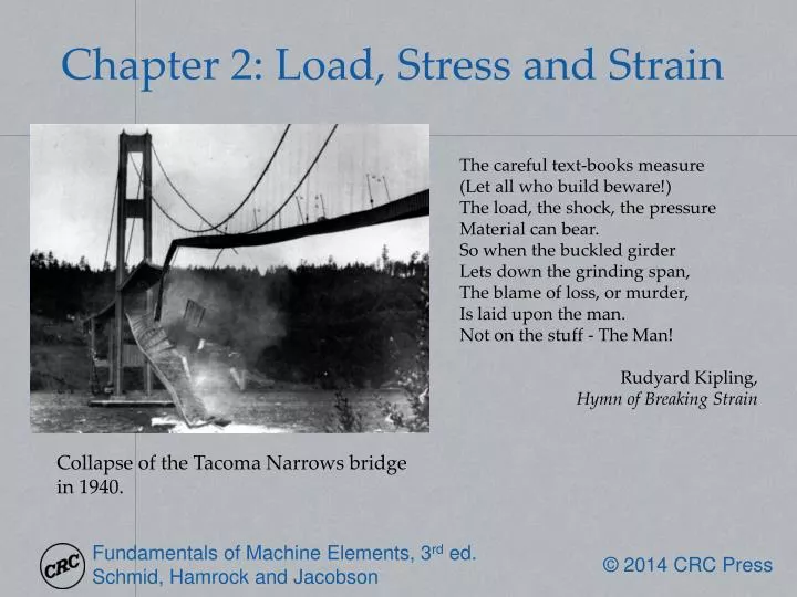
The careful text-books measure (Let all who build beware!) The load, the shock, the pressure Material can bear. So when the buckled girder Lets down the grinding span, The blame of loss, or murder, Is laid upon the man. Not on the stuff - The Man! Rudyard Kipling, Hymn of Breaking Strain Chapter 2: Load, Stress and Strain Collapse of the Tacoma Narrows bridge in 1940.
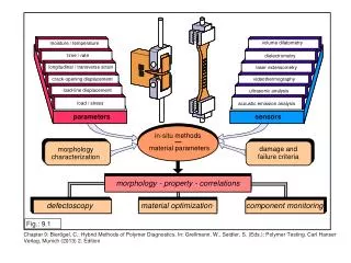
Design Procedure 2.1: Critical Section and Loading To establish the critical section and the critical loading, the designer: Considers the external loads applied to a machine (e.g., a gyroscope) Considers the external loads applied to an element within the machine (e.g., a ball bearing) Locates the critical section within the machine element (e.g., the inner race) Determines the loading at the critical section (e.g., contact stresses)
Example 2.1: Simple Crane Figure 2.1: A schematic of a simple crane and applied forces considered in Example 2.1. (a) Assembly drawing; (b) free-body diagram of forces acting on the beam.
Load Classification Any applied load can be classified with respect to time in the following ways: Static load- Load is gradually applied and equilibrium is reached in a relatively short time. The structure experiences no dynamic effects. Sustained load- Load, such as the weight of a structure, is constant over a long time. Impact load- Load is rapidly applied. An impact load is usually attributed to an energy imparted to a system. Cyclic load- Load can vary and even reverse its direction and has a characteristic period with respect to time. The load can also be classified with respect to the area over which it is applied: Concentrated load- Load is applied to an area much smaller than the loaded member. Distributed load- Load is spread along a large area. An example would be the weight of books on a bookshelf.
Load Classification Figure 2.2: Load classified as to location and method of application. (a) Normal, tensile; (b) normal, compressive; (c) shear; (d) bending; (e) torsion; (f) combined.
Sign Conventions Figure 2.3: Sign conventions used in bending. (a) Positive moment leads to a tensile stress in the positive y-direction; (b) positive moment acts in a positive direction on a positive face. The sign convention shown in (b) will be used in this book.
Supports and Reactions Table 2.1: Four types of support with their corresponding reactions.
Example 2.3 Figure 2.4: Lever assembly and results. (a) Lever assembly; (b) results showing (1) normal, tensile, (2) shear, (3) bending, (4) torsion on section B of lever assembly.
Example 2.4 Figure 2.5: Ladder in contact with a house and the ground while having a painter on the ladder.
Example 2.5 Figure 2.6: Sphere and applied forces. (a) Sphere supported with wires from top and spring at bottom; (b) free-body diagram of forces acting on sphere.
Example 2.6 Figure 2.7: External rim brake and applied forces, considered in Example 2.6. (a) External rim brake; (b) external rim brake with forces acting on each part. (Linear dimensions are in millimeters.)
Beam Supports Figure 2.8: Three types of beam support. (a) Simply supported; (b) cantilevered; (c) overhanging.
Design Procedure 2.2: Drawing Shear and Moment Diagrams by the Method of Sections The procedure for drawing shear and moment diagrams by the method of sections is as follows: Draw a free-body diagram and determine all the support reactions. Resolve the forces into components acting perpendicular and parallel to the beam's axis. Choose a position, x, between the origin and the length of the beam, l, thus dividing the beam into two segments. The origin is chosen at the beam's left end to ensure that any xchosen will be positive. Draw a free-body diagram of the two segments and use the equilibrium equations to determine the transverse shear force, V, and the moment, M. Plot the shear and moment functions versus x. Note the location of the maximum moment. Generally, it is convenient to show the shear and moment diagrams directly below the free-body diagram of the beam. Additional sections can be taken as necessary to fully quantify the shear and moment diagrams.
Example 2.7 Figure 2.9: Simply supported bar. (a) Midlength load and reactions; (b) free-body diagram for 0 < x < l/2; (c) free-body diagram for l/2 ≤x ≤ l; (d) shear and moment diagrams.
Example 2.8 Figure 2.10: Beam for Example 2.8. (a) Applied loads and reactions; (b) Shear diagram with areas indicated, and moment diagram with maximum and minimum values indicated.
Design Procedure 2.3: Singularity Functions Some general rules relating to singularity functions are: If n> 0 and the expression inside the angular brackets is positive (i.e., x ≥ a), then fn(x) = (x – a)n. Note that the angular brackets to the right of the equal sign in Eq.~(2.6) are now parentheses. If n> 0 and the expression inside the angular brackets is negative (i.e., x< a), then fn(x) = 0. If n< 0, then fn(x)= 0. If n= 0, then fn(x)= 1 when x ≥ aand fn(x)= 0 when x< a. If n ≥ 0, the integration rule is Note that this is the same as if there were parentheses instead of angular brackets. If n< 0, the integration rule is When n ≥ 1, then
Design Procedure 2.4: Shear and Moment Diagrams by Singularity Functions The procedure for drawing the shear and moment diagrams by making use of singularity functions is as follows: Draw a free-body diagram with all the applied distributed and concentrated loads acting on the beam, and determine all support reactions. Resolve the forces into components acting perpendicular and parallel to the beam's axis. Write an expression for the load intensity function q(x) that describes all the singularities acting on the beam. Use Table 2.2 as a reference, and make sure to “turn off” singularity functions for distributed loads and the like that do not extend across the full length of the beam. Integrate the negative load intensity function over the beam length to get the shear force. Integrate the negative shear force distribution over the beam length to get the moment, in accordance with Eqs. (2.4) and (2.5). Draw shear and moment diagrams from the expressions developed.
Singularity Functions Table 2.2: Singularity and load intensity functions with corresponding graphs and expressions.
Example 2.9 Figure 2.11: Beam for Example 2.8. (a) Applied loads and reactions; (b) Shear diagram with areas indicated, and moment diagram with maximum and minimum values indicated.
Example 2.10 Figure 2.12: Simply supported beam examined in Example 2.10. (a) Forces acting on beam when P1= 8 kN, P2= 5 kN; wo= 4 kN/m; l= 12 m; (b) free-body diagram showing resulting forces; (c) shear and (d) moment diagrams.
Example 2.11 Figure 2.13: Figures used in Example 2.11. (a) Load assembly drawing; (b) free-body diagram.
3D Stress Element Normal stress: Stress tensor: Figure 2.14: Stress element showing general state of three-dimensional stress with origin placed in center of element.
2D Stress Element Figure 2.15: Stress element showing two-dimensional state of stress. (a) Three-dimensional view; (b) plane view.
Equivalent Stress States Figure 2.16: Illustration of equivalent stress states; (a) Stress element oriented in the direction of applied stress; (b) stress element oriented in different (arbitrary) direction.
Stress on an Oblique Plane Stress transformation equations: Figure 2.17: Stresses in an oblique plane at an angle φ.
Design Procedure 2.5: Mohr’s Circle The steps in constructing and using Mohr's circle in two dimensions are as follows: Calculate the plane stress state for any x-ycoordinate system so that σx, σy, and τxyare known. The center of the Mohr's circle can be placed at Two points diametrically opposite to each other on the circle correspond to the points (σx, -τxy) and (σy, τxy). Using the center and either point allows one to draw the circle. The radius of the circle can be calculated from stress transformation equations or through geometry by using the center and one point on the circle. For example, the radius is the distance between points (σx, -τxy) and the center, which directly leads to
Design Procedure 2.5: Mohr’s Circle (cont.) The principal stresses have the values σ1,2= center ± radius. The maximum shear stress equals the radius. The principal axes can be found by calculating the angle between the x-axis in the Mohr's circle plane and the point (σx, -τxy). The principal axes in the real plane are rotated one-half this angle in the same direction relative to the x-axis in the real plane. The stresses in an orientation rotated φfrom the x-axis in the real plane can be read by traversing an arc of 2φin the same direction on the Mohr's circle from the reference points (σx, - τxy) and (σy, τxy). The new points on the circle correspond to the new stresses (σx’, - τxy) and (σy’, τxy), respectively.
Mohr’s Circle Center at: Radius: Figure 2.18: Mohr's circle diagram of Eqs. (2.13) and (2.14).
Example 2.14 Figure 2.19: Results from Example 2.14. (a) Mohr's circle diagram; (b) stress element for principal normal stress shown in x-ycoordinates; (c) stress element for principal shear stresses shown in x-ycoordinates.
Mohr’s Circle for Triaxial Stresses Figure 2.20: Mohr's circle for triaxial stress state. (a) Mohr's circle representation; (b) principal stresses on two planes.
Example 2.15 Figure 2.21: Mohr's circle diagrams for Example 2.15. (a) Triaxial stress state when σ1 = 234.3 MPa, σ2= 457 MPa and σ3 = 0; (b) biaxial stress state when σ1 = 307.6 MPa and σ2 = -27.6 MPa; (c) triaxial stress state when σ1 = 307.6 MPa, σ2 = 0, and σ3 = -27.6 MPa.
Octahedral Stresses Figure 2.22: Stresses acting on octahedral planes. (a) General state of stress. (b) normal stress; (c) octahedral shear stress. Octahedral stresses:
Normal Strain Normal strain: Figure 2.23: Normal strain of cubic element subjected to uniform tension in x-direction. (a) Three-dimensional view; (b) two-dimensional (or plane) view.
Shear Strain Figure 2.24: Shear strain of cubic element subjected to shear stress. (a) Three-dimensional view; (b) two-dimensional (or plane) view.
Plane Strain Element Figure 2.25: Graphical depiction of plane strain element. (a) Normal strain εx; (b) normal strain εy; and (c) shear strain γxy.
Example 2.18 Figure 2.26: Strain gage rosette used in Example 2.18.