Download
1 / 31
320 likes | 452 Views
Tangent linear and adjoint models for variational data assimilation. Angela Benedetti with contributions from: Marta Janiskov á, Philippe Lopez, Lars Isaksen , Gabor Radnoti and Yannick Tremolet. Introduction.

E N D
Tangent linear and adjoint models for variational data assimilation Angela Benedetti with contributions from: Marta Janisková, Philippe Lopez, Lars Isaksen, Gabor Radnoti and YannickTremolet
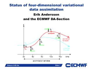
Introduction 4D-Var is based on minimization of a cost function which measures the distance between the model with respect to the observations and with respect to the background state The cost function and its gradient are needed in the minimization. The tangent linear model provides a computationally efficient (although approximate) way to calculate the model trajectory, and from it the cost function. The adjoint model is a very efficient tool to compute the gradient of the cost function. Overview: Brief introduction to 4D-Var with focus on TL/AD aspects General definitions of Tangent Linear and Adjoint models and why they are extremely useful in variational assimilation Writing TL and AD models Testing them Automatic differentiation software (more on this in the afternoon)
4D-Var In 4D-Var the cost function can be expressed as follows: Bbackground error covariance matrix, Robservation error covariance matrix (instrumental + interpolation + observation operator error), Mforward nonlinear forecast model (time evolution of the model state, index i), H observation operator (model space observation space). H’T = adjoint of observation operator and M’T = adjoint of forecast model.
Incremental 4D-Var at ECMWF • In incremental 4D-Var, the cost function is minimized in terms of increments: with the model state defined at any timeti as: at t=0) is the trajectory around which the linearization is performed ( • 4D-Var cost function can then be approximated to the first order by: • where • is the so-called departure computed using the nonlinear model and observational operator. • The gradient of the cost function to be minimized is: and are the tangent linear models which are used in the computations of incremental updates during the minimization (iterative procedure). and are the adjoint models which are used to obtain the gradient of the cost function with respect to the initial condition.
Details on linearisation In the first order approximation, a perturbation of the control variable (initial condition) evolves according to the tangent linear model: where i is the time-step. The perturbation of the cost function around the initial state is: where is the linearised version of about and are the departures from observations.
Details of the linearisation (cnt.) The gradient of the cost function with respect to is given by: remembering that The optimal initial perturbation is obtained by finding the value of for which: The gradient of the cost function with respect to the initial condition is provided by the adjoint solution at time t=0.
Definition of adjoint operator For any linear operator there exist an adjoint operator such as: where is an inner scalar product and x, y are vectors (or functions) of the space where this product is defined. It can be shown that for the inner product defined in the Euclidean space : We will now show that the gradient of the cost function at time t=0 is provided by the solution of the adjoint equations at the same time:
Adjoint solution Usually the initial guess is chosen to be equal to the background so that the initial perturbation The gradient of the cost function is hence simplified as: We choose the solution of the adjoint system as follows: We then substitute progressively the solution into the expression for
Adjoint solution (cnt.) Finally, regrouping and remembering that and that and we obtain the following equality: The gradient of the cost function with respect to the control variable (initial condition) is obtained by a backward integration of the adjoint model.
Iterative steps in the 4D-Var Algorithm Integrate forward model gives . Integrate adjoint model backwards gives . If then stop. Compute descent direction (Newton, CG, …). Compute step size : Update initial condition:
Finding the minimum of cost function J iterative minimization procedure cost function J J(xb) Jmini model variable x2 model variable x1
An analysis cycle in 4D-Var • 1st ifstraj: • Non-linear model is used to compute the high-res • trajectory (T1279 operational, 12-h forecast) • High-res departures are computed at exact obs • time and location • Trajectory is interpolated at low res (T159) • 1st ifsmin (70 iterations): • Iterative minimization at T159 resolution • Tangent linear with simplified physics to calculate • the increments • The Adjoint is used to compute the gradient of the • cost function with respect to the departure in • initial condition • Analysis increment at initial time is interpolated • back linearly from low-res to high-res and it provides • a new initial state for the 2nd trajectory run • 2nd ifstraj: • repeat 1st ifstraj and interpolates at T255 resolution • 2nd ifsmin (30 iterations): • repeat 1st ifsmin at T255 • Last ifstraj: • Uses updated initial condition to run another 12-h • forecast and stores analysis departures in the • Observational Data Base (ODB) 2 minimizations in the old configuration Now 3 minimizations are operational!
Simple example of adjoint writing (cnt.) Often the adjoint variables in mathematical formulations are indicated with an asterisk Do not forget the last equation!!! That too is part of the adjoint! As an alternative to the matrix method, adjoint coding can be carried out using a line-by-line approach.
More practical examples on adjont coding: the Lorenz model where is the Prandtl number, the Rayleigh number, and the aspect ratio. is the intensity of convection, is the maximum temperature difference is the stratification change due to convection. Details on the Lorenz model can be found in the references.
The linear code in Fortran Linearize each line of the code one by one, and set dx/dt=y for simplicity: y(1) = -p*x(1) +p*x(2) :Nonlinear statement (1)yd(1) = -p*xd(1) +p*xd(2) :Tangent linear y(2) = x(1)*(r-x(3)) -x(2) :Nonlinear statement (2)yd(2) = xd(1)*(r-x(3)) -x(1)*xd(3) -xd(2) :Tangent linear …etc Remember that p, r, bare constants; x(1), x(2) and x(3) are the independent variables; y(1), y(2) and y(3) are the dependent variables. We chose the suffix “d” for the tangent linear variable for consistency with the automatic differentation software (TAPENADE) which we will use this afternoon. Adjoint variables are indicated with the suffix “b”. This is just a convention. Note that in the ECMWF Integrated Forecast System (IFS) the tangent linear and adjoint variables are indicated without any subscripts and the nonlinear trajectory (x) is indicated with the suffix “5” (x5).
Adjoint of one instruction We start from the tangent linear code: yd(1)=-p*xd(1)+p*xd(2) In matrix form, it can be written as: which can easily be transposed (asterisk indicates adjoint variables): The corresponding adjoint code in FORTRAN is: xb(1)=xb(1)-p*yb(1) xb(2)=xb(2)+p*yb(1) yb(1)=0
Adjoint of one instruction (II) We start again from the tangent linear code: yd(2)= xd(1)*(r-x(3))-xd(2)- x(1)*xd(3) In matrix form, it can be written as: These terms come from the trajectory! Needs to be stored in memory or recomputed which can easily be transposed (asterisk indicates transposition): The corresponding adjoint code in FORTRAN is: xb(1)=xb(1)+(r-x(3))*yb(2) xb(2)=xb(2)- yb(2) xb(3)=xb(3)- x(1)*yb(2) yb(2)=0
Trajectory • The trajectory has to be available. It can be: • saved which costs memory, • recomputed which costs CPU time. • Depending on the complexity of the code, one • option or the other is adopted (or a mixture • of the two options).
The Adjoint Code Property of adjoints (transposition): Application: where represents the line of the tangent linear model. The adjoint code is made of the transpose of each line of the tangent linear code in reverse order.
Adjoint of loops In the TL code for the Lorenz model we have: DO i=1,3 xd(i)=xd(i)+dt*yd(i) ENDDO dt is a constant for our purposes.This loop can be written explicitly: xd(1)=xd(1)+dt*yd(1) xd(2)=xd(2)+dt*yd(2) xd(3)=xd(3)+dt*yd(3) We can now transpose and reverse the lines to get the adjoint: yb(3)=yb(3)+dt*xb(3) yb(2)=yb(2)+dt*xb(2) yb(1)=yb(1)+dt*xb(1) which is equivalent to DO i=3,1,-1 !Reverse order of indeces! yb(i)=yb(i)+dt*xb(i) ENDDO
Conditional statements (“IF” statements) What we want is the adjoint of the statements which were actually executed in the direct model. We need to know which “branch” of the IF statement was executed The result of the conditional statement has to be stored: it is part of the trajectory !!!
Summary of basic rules for line-by-line adjoint coding (1) Adjoint statements are derived from tangent linear ones in a reversed order Order of operations is important when variable is updated! And do not forget to initialize local adjoint variables to zero !
Summary of basic rules for line-by-line adjoint coding (2) To save memory, the trajectory can be recomputed just before the adjoint calculations (again it depends on the complexity of the model). • The most common sources of error in adjoint coding are: • Pure coding errors • Forgotten initialization of local adjoint variables to zero • Mismatching trajectories in tangent linear and adjoint (even slightly) • Bad identification of trajectory updates
More remarks about adjoints The adjoint always exists and it is unique, assuming spaces of finite dimension. Hence, coding the adjoint does not raise questions about its existence, only questions of technical implementation. In the meteorological literature, the term adjoint is often improperly used to denote the adjoint of the tangent linear of a non-linear operator. In reality, the adjoint can be defined for any linear operator. One must be aware that discussions about the existence of the adjoint usually should address the existence of the tangent linear model. Without re-computation, the cost of the TL is usually about 1.5 times that of the non-linear code, the cost of the adjoint between 2 and 3 times. The tangent linear model is not strictly necessary to run 4D-Var (but it is in the incremental 4D-Var formulation in use operationally at ECMWF). It is also needed as an intermediate step to write and test the adjoint.
Test for tangent linear model machine precision reached Perturbation scaling factor
Test for adjoint model The adjoint test is truly unforgiving. If you do not have a ratio of the norm close to 1 within the precision of the machine, you know there is a bug in your adjoint. At the end of your debugging you will have a perfect adjoint (although you may still have an imperfect tangent linear!) More on this in the afternoon!
Test of adjoint in practice…(more on this in the afternoon) • Compute perturbed variable (y) using perturbation in input variables (x,z) with the tangent linear code • Compute TL norm: • Call adjoint routine to obtain gradients in x and z with respect to initial perturbation in x and z from perturbation in y. • Compute the norm from the adjoint calculation, using unperturbed state and gradients: • According to the test of adjoint NORM_TL must be equal to NORM_AD to the machine precision!
Automatic differentiation Because of the strict rules of tangent linear and adjoint coding, automatic differentiation is possible. Existing tools: TAF (TAMC), TAPENADE (Odyssée), ... Reverse the order of instructions, Transpose instructions instantly without typos !!! Especially good in deriving tangent linear codes! There are still unresolved issues: It is NOT a black box tool, Cannot handle non-differentiable instructions (TL is wrong), Can create huge arrays to store the trajectory, The codes often need to be cleaned-up and optimised.
Variational data assimilation: Lorenc, A., 1986, Quarterly Journal of the Royal Meteorological Society, 112, 1177-1194. Courtier, P. et al., 1994, Quarterly Journal of the Royal Meteorological Society, 120, 1367-1387. Rabier, F. et al., 2000, Quarterly Journal of the Royal Meteorological Society, 126, 1143-1170. The adjoint technique: Errico, R.M., 1997, Bulletin of the American Meteorological Society, 78, 2577-2591. Tangent-linear approximation: Errico, R.M. et al., 1993, Tellus, 45A, 462-477. Errico, R.M., and K. Reader, 1999, Quarterly Journal of the Royal Meteorological Society, 125, 169-195. Janisková, M. et al., 1999, Monthly Weather Review, 127, 26-45. Mahfouf, J.-F., 1999, Tellus, 51A, 147-166. Lorenz model: X. Y. Huang and X. Yang. Variational data assimilation with the Lorenz model. Technical Report 26, HIRLAM, April 1996. Available on ftp site (see notes for practical session). E. Lorenz. Deterministic nonperiodic flow. J. Atmos. Sci., 20:130-141, 1963. Automatic differentiation: Giering R., Tangent Linear and Adjoint Model Compiler, Users Manual Center for Global Change Sciences, Department of Earth, Atmospheric, and PlanetaryScience,MIT,1997 Giering R. and T. Kaminski, Recipes for Adjoint Code Construction, ACM Transactions on Mathematical Software, 1998 TAMC: http://www.autodiff.org/ TAPENADE: http://www-sop.inria.fr/tropics/tapenade.html Sensitivity studies using the adjoint technique Janiskova, M. and J.-J. Morcrette., 2005. Investigation of the sensitivity of the ECMWF radiation scheme to input parameters using adjoint technique. Quart. J. Roy. Meteor. Soc., 131,1975-1996. Useful References