Download
1 / 51

E N D
Real Time PCR M.Prasad Naidu MSc Medical Biochemistry, Ph.D,.
Traditional PCR (semiquantitative) 1 2 4 8 2 denaturation 95°C annealing 60°C n cycles extension 72°C n Gel electroforesis Specificity determined by 2 primers
Precise Ct Traditional PCR (semiquantitative) Plateau phase Variable PCR Plateau(taq efficiency decreases, reagents get limiting, decreased denaturation efficiency, …) Amplification Plot of 96 Sample Replicates Plateau phase
Principles of quantitative PCR • Monitors the progress of the PCR as it occurs (in “real time”) by reading fluorescence intensities after each cycle. Intensities are proportional to the number of amplicons generated • Samples are characterized by the point in time during cycling, when amplification is first detected (more starting material sooner an increase in fluorescence) • For allelic discrimination, endpoint assays are used • Temperature protocol: also > 30 cycles 30” 95°C 30” 60°C 30” 72°C/60°C
Exponential growth phase = linear part in logarithmic graphic 1 2 4 8 2 n cycles n
CHEMISTRY • SYBR green • Taqman probes • Molecular Beacons • Scorpion primers
CHEMISTRY 1) SYBR green I • intercalating dye, binds double strand DNA • More sensitive than EtBr • Specificity determined by 2 primers • No probe required (lower costs) • Also detection of aspecific products melting curve after PCR reaction • Only singleplex • No allelic discrimination possible
CHEMISTRY Dissociation Curve 1) SYBR green I • Dissociation Protocol can be added to the thermal cycling parameters • Allows detection of non-specific products 95°C 15s 95°C 60°C 1min 60°C 20s cycle 40 20min
SYBR dissociates from ds amplicon baseline Raw Data View Dissociation Curve Natural decrease in SYBR fluorescence Tm = temperature when 50% dissociated
Target amplicon Dissociation Curve Derivative Data View Tm = temperature when 50% dissociated
Dissociation Curve Example: Presence of Primer Dimers Product Primer dimers or aspecific product
CHEMISTRY 2) Taqman probe Mechanism: fluorescence resonance energy transfer (FRET) Annealing and polymerization Strand displacement • Cleavage (5’ nuclease activity of taq DNA • polymerase) • Increase of reporter signal proportional to amount of amplicon produced • Removes probe from target strand Cleavage
CHEMISTRY 2) Taqman probe • Two primers + a fluorogenic probe determine specificity • No detection of aspecific products • No melting curve needed (faster) • Can be used for allelic discrimination • Multiplex • Synthesis of different probes required for different sequences
Rox Fam Vic/Joe Tamra CHEMISTRY 2) Taqman probe Multiplex reactions possible • Reporters: FAM,TET,VIC,JOE • Quenchers: TAMRA, MGB • Passive reference: ROX normalizes for non-PCR-related fluorescence fluctuations occurring well-to-well (concentration or volume differences) Emission Profiles of Various Fluorophores: Spectral compensation necessary
DEFINITIONS • Baseline • Threshold • Rn • Ct Baseline = Basal level of fluorescence defined during the initial cycles of PCR (background fluorescence). Threshold = Fixed fluorescence level set above the baseline (statistical cutoff based upon background fluorescence). Rn = normalized Reporter signal, level of fluorescence detected during PCR. Calculated by dividing probe reporter dye signal by passive reference signal (ROX). Ct = threshold Cycle, PCR cycle at which an increase in reporter fluorescence above a baseline signal is first detected (cycle when fluorescence crosses the threshold).
Ct Ct Ct Ct DEFINITIONS • Setting baseline and threshold (exponential growth) determining Ct (threshold cycle) of each sample • Ct is the cycle number at which the fluorescence passes the threshold EXAMPLE GRAPHIC threshold baseline
Advantages of using Real-Time PCR • COLLECTS DATA IN THE EXPONENTIAL GROWTH PHASE • REAL TIME: permanent record of amplification • INCREASED DYNAMIC RANGE of detection • LESS RNA NEEDED Requirement of 1000-fold less RNA than conventional assays • FAST: No-post PCR processing • SENSIBLE: Detection is capable down to a 2-fold change
APPLICATIONS • Real time detection: • Quantitation of gene expression • Quantitation of RNA, DNA, cDNA • Viral quantitation • … • Endpoint detection: • Allelic discrimination (SNP genotyping) • Plus/minus studies • Pathogen detection • …
APPLICATIONS • Real time detection: • Quantitation of gene expression • Quantitation of RNA, DNA, cDNA • Viral quantitation • … • Endpoint detection: • Allelic discrimination (SNP genotyping) • Plus/minus studies • Pathogen detection • …
Quantification • Absolute quantification (result in copy number): virus copy number,… 1.Calculation by standard curve • Relative quantification (result is given as relative to the reference sample): gene expression,… 2.Calculation by standard curve 3. Use of comparative Ct method
APPLICATIONS • Real time detection: • Quantitation of gene expression • Quantitation of RNA, DNA, cDNA • Viral quantitation • … • Endpoint detection: • Allelic discrimination (SNP genotyping) • Plus/minus studies • Pathogen detection • …
Absolute Quantitation: Standard Curve
Standard curve Quantify sample by spectrofotometry, make dilution curve
Standard curve Ct Ct= 29.7 Log Qty Log Qty = 3.28
Relative Quantitation: Standard Curve
Relative quantitation: example • Cells: • Basal conditions • Treatment IL6 3h • Treatment OSM 3h • Define expression of gene of interest (SOCS3) upon treatment, relative to expression at basal conditions
We need an endogenous control to normalize for the amount of starting material in the tube ! • β-actin • GAPDH • 18S and others The perfect standard does not exist; choose the best control for your system ratio target gene (experimental/control) = fold change in target gene (exp/control) fold change in reference gene (exp/control)
Relative quantitation: example • Make dilution series of a sample • Read SOCS3 levels of standard curve and unknown samples • Read 18S levels of standard curve and unknown samples; • Choose a sample (cells in basal conditions) as calibrator If level SOCS3 (sample IL6 45 min)/ level SOCS3 (sample basal conditions)= 10x Level 18S (sample IL6 45 min)/ level 18S (sample basal conditions)= 2x Then the level of SOCS3 after IL6 treatment is 5x higher than at basal conditions
Relative Quantitation: ΔΔCt method
ΔΔCt method Principle: Samples that differ by a factor of 2 in the original concentration would be theoretically expected to be 1 cycle apart. Samples that differ by a factor of 10 (as in our dilution series) would be ~3.3 cycles apart. Example 1: Ct(A)= 30 Ct(B)= 31 RQ = 21 = 2 Example 2: Ct(A)= 30 Ct(B)= 33,3 RQ = 23.3 = 10 CT (sample) - CT (basal) Relative Quantity = 2
BUT: calibrator sample 8 targ 4 ref 12 targ 2 ref ratio = fold change in target gene (sample) fold change in reference gene (sample) fold change in target gene (calibrator) fold change in reference gene (calibrator) CT(sample) = CT (Target) - CT (Reference) CT(calibrator) = CT (Target) - CT (Reference) CT = CT (Sample) - CT (Calibrator) Relative Quantity = 2 -ΔΔCt
ΔΔCt method: Example • Example 1: • CT(sample) = CT (Target) - CT (Reference) DCt(ctrl SOCS3)= 27-20 = 7 • DCt(tr SOCS3)= 24-20 = 4 • CT = CT (Sample) - CT (Calibrator) DDCt = 4 – 7 = -3 RQ = 23 = 8 Note: Also Ct(tr SOCS3) – Ct(ctrl SOCS3) = 27-24= 3 because starting conc was equal (equal 18S) SOCS3 expression in treated sample is 8 times higher than in control sample. ctrl 18S ctrl SOCS3 ctrl SOCS3 tr 18S tr 18S ctrl 18S tr SOCS3 tr SOCS3
ΔΔCt method: Example • Example 2: • CT(sample) = CT (Target) - CT (Reference) DCt(ctrl SOCS3)= 28-16 = 12 • DCt(tr SOCS3)= 25-13 = 12 • CT = CT (Sample) - CT (Calibrator) DDCt = 12 – 12 = 0 RQ = 20 = 1 no difference in SOCS3 expression in treated and control sample! ctrl 18S ctrl SOCS3 ctrl SOCS3 tr 18S tr 18S ctrl 18S tr SOCS3 tr SOCS3
ΔΔCt method • no need for dilution series less material needed, faster BUT: amplification efficiency of target and endogenous control must be comparable
ΔΔCt method Efficiency of amplification Changes in efficiency change the slope when you use the logarithmic scale.
30 25 20 15 10 Validation of efficiency • equal efficiency or equal slopes for target and • endogenous control • - Acceptible slope = 3.2 - 3.8 (Efficiency 83 – 105 %) Target 35 Target y = - 4. 586x + 24.889 Effic = 67 % Endogenous control y = - 3.3683x + 36.009 Effic = 98 % Value t C D y = - 3.3276x + 27.712 Effic = 100 % 0 2 4 6 8 1 0 Log [Input mRNA]
ΔΔCt method Does the target have a similar amplification efficiency to the endogenous control? YES NO Ct method Standard Curves
Primers and probe design Primer Tm 58 - 60ºC 20 - 80% GC Length 9 - 40 <2ºC difference in Tm between the two primers Maximum of 2 G or C at 3’ end Amplicon 50 - 150 bp in length As close to the probe as possible without overlapping Probe Tm 10ºC higher than Primer Tm (7ºC for Allelic Discrimination) 20 - 80% GC Length 9 - 40 bases No G on the 5’end <4 contiguous G’s Must not have more G’s than C’s
Primers and probe design Primer Concentration Optimization MATRIX FORWARD REVERSE 50nM 300nM 900nM 50nM 50/50 300/50 900/50 300nM 50/300 300/300 900/300 900nM 50/900 300/900 900/900
Primer Optimisation for SYBR Green I • Perform 50/300/900nM primer matrix: Choose the optimal primer concentration • Lowest Ct • Highest Rn • No amplification in negative control Probe Optimisation (Taqman) • Increase probe concentration from 50nM to 300nM • Lowest Ct without excess probe
Multiplex reactions • Primers and probes for both target gene (SOCS3) and reference gene (18S) in the same tube • Primers for reference gene (18S) must be limited target gene 18 S
APPLICATIONS • Real time detection: • Quantitation of gene expression • Quantitation of RNA, DNA, cDNA • Viral quantitation • … • Endpoint detection: • Allelic discrimination (SNP genotyping) • Plus/minus studies • Pathogen detection • …
End Point Real Time Assays +/- Allelic Discrimination (SNPs) Assays +/- Alelic Discrimination (SNPs) Absolute Quantitation Relative Quantitation Absolute Quantitation Relative Quantitation ALLELIC DISCRIMINATION End point detection
Allele 1 Tamra Tamra™ VIC FAM Mismatch Perfect match Allele 2 Tamra Tamra FAM VIC Mismatch Perfect match ALLELIC DISCRIMINATION Principle: 2 primers, 2 probes FAM™-labelled probe is specific for Allele 1 VIC™-labelled probe is specific for Allele 2
ALLELIC DISCRIMINATION Mechanism • relies on competition between the two probes • Tm of the mismatched probe < Tm of perfectly matched probe Tamra™ VIC™ Tamra FAM™ Allele 1 Allele 1 Incorrect Probe Correct Probe Tm = 55ºC Tm = 65ºC Annealing/extension temperature of 60°C allows binding and cleavage of correct probe and destabilisation of incorrect probe
ALLELIC DISCRIMINATION Typical output FAM VIC Allele 1 Allele 2 VIC FAM homozygote for allele 1 homozygote for allele 2 FAM VIC Allele 1&2 heterozygote
ALLELIC DISCRIMINATION Typical output