Download
1 / 56
560 likes | 725 Views
More on Coordinate Systems. We have been using the coordinate system of the screen window (in pixels). The range is from 0 (left) to some value screenWidth – 1 in x , and from 0 (usually top) to some value screenHeight –1 in y . We can use only positive values of x and y.

E N D
More on Coordinate Systems • We have been using the coordinate system of the screen window (in pixels). • The range is from 0 (left) to some value screenWidth – 1 in x, and from 0 (usually top) to some value screenHeight –1 in y. • We can use only positive values of x and y. • The values must have a large range (several hundred pixels) to get a reasonable size drawing.
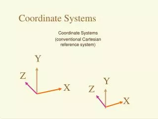
Coordinate Systems (2) • It may be much more natural to think in terms of x varying from, say, -1 to 1, and y varying from –100.0 to 20.0. • We want to separate the coordinates we use in a program to describe the geometrical object from the coordinates we use to size and position the pictures of the objects on the display. • Description is usually referred to as a modeling task, and displaying pictures as a viewing task.
Coordinate Systems (3) • The space in which objects are described is called world coordinates (the numbers used for x and y are those in the world, where the objects are defined). • World coordinates use the Cartesian xy-coordinate system used in mathematics, based on whatever units are convenient.
Coordinate Systems (4) • We define a rectangular world window in these world coordinates. • The world window specifies which part of the world should be drawn: whichever part lies inside the window should be drawn, and whichever part lies outside should be clipped away and not drawn. • OpenGL does the clipping automatically.
Coordinate Systems (5) • In addition, we define a rectangular viewport in the screen window on the display. • A mapping (consisting of scalings [change size] and translations [move object]) between the world window and the viewport is established by OpenGL. • The objects inside the world window appear automatically at proper sizes and locations inside the viewport (in screen coordinates, which are pixel coordinates on the display).
Coordinate Systems Example • We want to graph • Sinc(0) = 1 by definition. Interesting parts of the function are in -4.0 ≤ x ≤ 4.0.
Coordinate Systems Example (2) • The program which graphs this function is given in Fig. 3.3. • The function setWindow sets the world window size: void setWindow(GLdouble left, GLdouble right, GLdouble bottom, GLdouble top) { glMatrixMode(GL_PROJECTION); glLoadIdentity(); gluOrtho2D(left, right, bottom, top);}
Coordinate Systems Example (3) • The function setViewport sets the screen viewport size: void setViewport(GLint left, GLint right, GLint bottom, GLint top) { glViewport(left, bottom, right - left, top - bottom);} • Calls: setWindow(-5.0, 5.0, -0.3, 1.0); • setViewport(0, 640, 0, 480);
Windows and Viewports • We use natural coordinates for what we are drawing (the world window). • OpenGL converts our coordinates to screen coordinates when we set up a screen window and a viewport. The viewport may be smaller than the screen window. The default viewport is the entire screen window. • The conversion requires scaling and shifting: mapping the world window to the screen window and the viewport.
Mapping Windows • Windows are described by their left, top, right, and bottom values, w.l, w.t, w.r, w.b. • Viewports are described by the same values: v.l, v.t, v.r, v.b, but in screen window coordinates.
Mapping (2) • We can map any aligned rectangle to any other aligned rectangle. • If the aspect ratios of the 2 rectangles are not the same, distortion will result.
Window-to-Viewport Mapping • We want our mapping to be proportional: for example, if x is ¼ of the way between the left and right world window boundaries, then the screen x (sx) should be ¼ of the way between the left and right viewport boundaries.
Window-to-Viewport Mapping (2) • This requirement forces our mapping to be linear. • sx= Ax + C, sy = B y + D • We require (sx – V.l)/(V.r – V.l) = (x – W.l)/(W.r – W.l), giving • sx = x*[(V.r-V.l)/(W.r-W.l)] + {V.l – W.l*[(V.r-V.l)/(W.r-W.l)]}, or A = (V.r-V.l)/(W.r-W.l), C = V.l – A*w.l
Window-to-Viewport Mapping (3) • We likewise require (sy – V.b)/(V.t – V.b) = (y – W.b)/(W.t – W.b), giving • B = (V.t-V.b)/(W.t-W.b), D = V.b – B*W.b • Summary: sx = A x + C, sy = B y + D, with
GL Functions To Create the Map • World window: void gluOrtho2D(GLdouble left, GLdouble right, GLdouble bottom, GLdouble top); • Viewport: void glViewport(GLint x, GLint y, GLint width, GLint height); • This sets the lower left corner of the viewport, along with its width and height.
GL Functions To Create the Map (2) • Because OpenGL uses matrices to set up all its transformations, the call to gluOrtho2D() must be preceded by two setup functions: glMatrixMode(GL_PROJECTION); and glLoadIdentity(); • setWindow() and setViewport() are useful code “wrappers”. • They simplify the process of creating the window and viewport.
Applications (continued) • Tiling A was set up by the following code: setWindow(0, 640.0, 0, 440.0); // set a fixed window for (int i = 0; i < 5; i++) // for each column for (int j = 0; j < 5; j++){ // for each row {glViewport (i*64, j*44,64, 44); // set the next viewport drawPolylineFile("dino.dat"); // draw it again } • Tiling B requires more effort: you can only turn a window upside down, not a viewport.
Applications (continued) • Code for Tiling B for (int i = 0; i < 5; i++) // for each column for (int j = 0; j < 5; j++){ // for each row if ((i + j) % 2 == 0){ setWindow(0.0, 640.0, 0.0, 440.0); } else { setWindow(0.0, 640.0, 440.0, 0.0); // upside-down } glViewport (i*64, j*44,64, 44); // no distortion drawPolylineFile("dino.dat"); }
Application: Clip, Zoom and Pan Clipping refers to viewing only the parts of an image that are in the window.
Application (continued) • The figure is a collection of concentric hexagons of various sizes, each rotated slightly with respect to the previous one. It is drawn by a function called hexSwirl (); • The figure showed 2 choices of world windows. • We can also use world windows for zooming and roaming (panning).
Zooming and Panning • To zoom, we pick a concentric set of windows of decreasing size and display them from outside in.
Zooming and Roaming (2) • The animation of the zoom will probably not be very smooth. We want to look at one drawing while the next one is drawn, and then switch to the new drawing. • We use glutInitDisplayMode (GLUT_DOUBLE | GLUT_RGB); //gives us 2 buffers, one to look at and one to draw in • We add glutSwapBuffers(); after the call to hexSwirl (); // change to the new drawing
Roaming (Panning) • To roam, or pan, we move a viewport through various portions of the world. This is easily accomplished by translating the window to a new position. • What sequence of windows would you want in order to roam through the image?
Resizing the Screen Window • Users are free to alter the size and aspect ratio of the screen window. • You may want GL to handle this event so that your drawing does not get distorted. • Register the reshape function: glutReshapeFunc (myReshape); • Void myReshape (GLsizei W, GLsizei H); collects the new width and height for the window.
Preserving Aspect Ratio • We want the largest viewport which preserves the aspect ratio R of the world window. • Suppose the screen window has width W and height H: • If R > W/H, the viewport should be width W and height W/R • If R < W/H, the viewport should be width H*R and height H • What happens if R = W/H?
Clipping Lines • We want to draw only the parts of lines that are inside the world window. • To do this, we need to replace line portions outside the window by lines along the window boundaries. The process is called clipping the lines.
Clipping (2) • The method we will use is called Cohen-Sutherland clipping. • There are 2 trivial cases: a line AB totally inside the window, which we draw all of, and a line CD totally outside the window, which we do not draw at all.
Clipping (3) • For all lines, we give each endpoint of the line a code specifying where it lies relative to the window W:
Clipping (4) • The diagram below shows Boolean codes for the 9 possible regions the endpoint lies in (left, above, below, right).
Clipping (5) • A line consists of 2 endpoints (vertices), P1 and P2. If we do not have a trivial case, we must alter the vertices to the points where the line intersects the window boundaries (replace P1 by A).
Clipping (6) • In the diagram, d/dely = e/delx (similar triangles). • Obviously, A.x = W.r. • Also, delx = p1.x – p2.x, dely = p1.y – p2.y and e = p1.x – W.r. • So A.y = p1.y – d.
A Line Needing 4 Clips • The equation of the line is y = x * (p1.y – p2.y)/(p1.x – p2.x) + p2.y = mx + p2.y. • The intersection B with the top window boundary is at x where y = W.t, or x = (W.t – p2.y)/m. • The intersection A with the right boundary is y where x = W.r, or y = m*W.r + p2.y.
Clipping Pseudocode • Complete pseudocode for the Cohen-Sutherland Line Clipper is shown in Fig. 3.21.
Drawing Regular Polygons, Circles, and Arcs • A polygon is regular if it is simple, if all its sides have equal length, and if adjacent sides meet at equal interior angles. • A polygon is simple if no two of its edges cross each other. More precisely, only adjacent edges can touch and only at their shared endpoint. • We give the name n-gon to a regular polygon having n sides; familiar examples are the 4-gon (a square), an 8-gon (a regular octagon) and so on.
Drawing Circles and Arcs • Two methods: • The center is given, along with a point on the circle. • Here drawCircle( IntPoint center, int radius) can be used as soon as the radius is known. If c is the center and p is the given point on the circle, the radius is simply the distance from c to p, found using the usual Pythagorean Theorem.
Drawing Circles and Arcs • Three points are given through which the circle must pass. • It is known that a unique circle passes through any three points that don't lie in a straight line. • Finding the center and radius of this circle is discussed in Chapter 4.
Successive Refinement of Curves • Very complex curves can be fashioned recursively by repeatedly “refining” a simple curve. • Example: the Koch curve, which produces an infinitely long line within a region of finite area.
Koch Curves • Successive generations of the Koch curve are denoted K0, K1, K2,… • The 0-th generation shape K0 is just a horizontal line of length 1. • The curve K1 is created by dividing the line K0 into three equal parts, and replacing the middle section with a triangular bump having sides of length 1/ 3. The total line length is evidently 4 / 3.
Koch Curves (2) • The second-order curve K2 is formed by building a bump on each of the four line segments of K1.
Koch Snowflake (3 joined curves) • Perimeter: the i-th generation shape Si is three times the length of a simple Koch curve, 3(4/3)i, which grows forever as i increases. • Area inside the Koch snowflake: grows quite slowly, and in the limit, the area of S∞ is only 8/5 the area of S0.
Parametric Curves • Three forms of equation for a given curve: • Explicit: e.g., y = m*x + b • Implicit: F(x, y) = 0; e.g., y – m*x –b = 0 • Parametric: x = x(t), y = y(t), t a parameter; frequently, 0 ≤ t ≤ 1. E.g., P = P1*(1-t) + P2*t. • P1 and P2 are 2D points with x and y values. The parametric form is x = x1*(1-t) + x2*t and y = y1*(1-t) + y2*t.
Specific Parametric Forms • line: x = x1*(1-t) + x2*t and y = y1*(1-t) + y2*t • circle: x = r*cos(2π t), y = r*sin(2π t) • ellipse: x = W*r*cos(2π t), y = H*r*sin(2π t) • W and H are half-width and half-height.
Finding Implicit Form from Parametric Form • Combine the x(t) and y(t) equations to eliminate t. • Example: ellipse: x = W*r*cos(2π t), y = H*r*sin(2π t) • X2 = W2r2cos2(2π t), y2 = H2r2sin2(2π t). • Dividing by the W or H factors and adding gives (x/W)2 + (y/H)2 = 1, the implicit form.
Drawing Parametric Curves • For a curve C with the parametric form P(t) = (x(t), y(t)) as t varies from 0 to T, we use samples of P(t) at closely spaced instants.
Drawing Parametric Curves (2) • The position Pi = P(ti) = (x(ti), y(ti)) is calculated for a sequence {ti} of times. • The curve P(t) is approximated by the polyline based on this sequence of points Pi.