Abstract

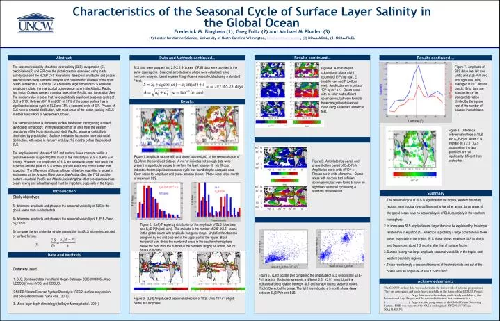
1. Characteristics of the Seasonal Cycle of Surface Layer Salinity in the Global OceanFrederick M. Bingham (1), Greg Foltz (2) and Michael McPhaden (3) (1) Center for Marine Science,University of North Carolina Wilmington, binghamf@uncw.edu, (2) NOAA/AOML, (3) NOAA/PMEL Results continued… Abstract Data and Methods continued… Results continued... The seasonal variability of surface layer salinity (SLS), evaporation (E), precipitation (P) and E-P over the global ocean is examined using in situ salinity data and the NCEP CFS Reanalysis. Seasonal amplitudes and phases are calculated using harmonic analysis and presented in all areas of the open ocean between 60°S and 60°N. Areas with large amplitude SLS seasonal variations include: the intertropical convergence zone in the Atlantic, Pacific and Indian Oceans; western marginal seas of the Pacific; and the Arabian Sea. The median value in areas that have statistically significant seasonal cycles of SLS is 0.19. Between 60°S and 60°N, 37% of the ocean surface has a significant seasonal cycle of SLS and 75% a seasonal cycle of E-P. Phases of SLS have a bimodal distribution, with most areas of the ocean peaking in SLS in either March/April or September/October. The same calculation is done with surface freshwater forcing using a mixed-layer depth climatology. With the exception of an area near the western boundaries of the North Atlantic and North Pacific, seasonal variability is dominated by precipitation. Surface freshwater fluxes also have a bimodal distribution, with peaks in January and July, 1-2 months before the peaks of SLS. The amplitudes and phases of SLS and surface fluxes compare well in a qualitative sense, suggesting that much of the variability in SLS is due to E-P forcing. However, the amplitudes of SLS are somewhat larger than would be expected and the peak of SLS comes typically about one month earlier than expected. The differences of the amplitudes of the two quantities is largest in such areas as the Amazon River plume, the Arabian Sea, the ITCZ and the eastern equatorial Pacific and Atlantic, indicating that other processes such as ocean mixing and lateral transport must be important, especially in the tropics. Figure 7. Amplitude of SLS (blue line, left axis units) and S0(E-P)/h (red line, right axis units) averaged in 10° latitude bands. Error bars are standard error, i.e. standard deviation divided by the square root of the number of squares in each band. SLS data were grouped into 2.5oX 2.5o boxes. CFSR data were provided in the same size regions. Seasonal amplitude and phase were calculated using harmonic analysis. Least squares fit significance was calculated using a standard F-test. Figure 4. Amplitude (left column) and phase (right column) of E-P (top row), E (middle row) and P (bottom row). Amplitudes are in units of 10-4 kg m-2 s-1. Ocean areas with no color had sufficient observations, but were found to have no significant seasonal cycle using a standard statistical test. Results Figure 8. Difference between amplitude of SLS and S0(E-P)/h. A red 'x' is overlaid on a 2.5°X2.5° square when the two quantities are not significantly different from each other. Figure 1. Amplitude (above left) and phase (above right) of the seasonal cycle of SLS from the combined dataset. A red “x” indicates not enough data were present in a particular square to perform the least squares fit. No fill color indicates that no significant seasonal cycle was found despite adequate data. Color scales for amplitude and phase are also shown. Phase scale is the month of maximum SLS. Figure 5. Amplitude (top panel) and phase (bottom panel) of S0(E-P)/h. Amplitudes are in units of 10-8 s-1. Phases are in units of months. Ocean areas with no color had sufficient observations, but were found to have no significant seasonal cycle using a standard statistical test. Introduction Study objectives To determine amplitude and phase of the seasonal variability of SLS in the global ocean from available data To determine amplitude and phase of the seasonal variability of E, P, E-P and S0(E-P)/h. To compare the two under the simple assumption that SLS is largely controlled by surface forcing. (1) Summary The seasonal cycle of SLS is significant in the tropics, western boundary regions, near tropical river outflows and a few other areas. Large areas of the global ocean have no seasonal cycle of SLS, especially in the southern hemisphere. In some area SLS amplitudes are larger than can be explained by the simple relationship in equation (1). Advection is probably a large contributor in these areas, especially in the tropics. SLS phase shows maximum SLS in March and September, about 1-2 months after that of surface forcing. Surface forcing has large amplitude seasonal variability in the tropics and western boundary regions. These results imply a seasonal transport of freshwater into and out of the ocean with an amplitude of about 19X103 km3. Figure 2. (Left) Frequency distribution of the amplitude of SLS (blue bars) and S0(E-P)/h (red bars). The ordinate is the number of 2.5°X2.5° areas in the global ocean with amplitude in a given range. Units for the abscissa are given by red and blue text in the upper part of the figure. Black horizontal bars divide the number of areas in the southern hemisphere below the bars from the number in the northern. (Right) As above, but for phase in months. Data and Methods Datasets used 1. SLS: Combined data from World Ocean Database 2005 (WOD05), Argo, LEGOS (French VOS)‏ and GOSUD. 2.NCEP Climate Forecast System Reanalysis (CFSR) surface evaporation and precipitation fluxes (Saha et al., 2010)‏. 3. Mixed-layer depth climatology (de Boyer Montegut et al., 2004) Figure 6. (Left) Scatter plot comparing the amplitude of SLS (y-axis) and S0(E-P)/h (x-axis). Each dot represents a different 2.5°X2.5° area. Light line indicates a direct relation between SLS and surface forcing seasonal cycles. (Right) Same, but for phase. The light line indicates a 3 month phase delay between S0(E-P)/h and SLS. Acknowledgements The GOSUD surface data were collected in the framework of national programmes. They are aggregated and made freely available in the frame of the GOSUD Project: http://www.gosud.org. Argo data were collected and made freely available by the International Argo Project and the national initiatives that contribute to it (http://www.argo.net). Argo is a pilot programme of the Global Ocean Observing System. FMB was supported by NASA under grants NNX09AU70G and NNX11AE83G. Figure 3. (Left) Amplitude of seasonal advection of SLS. Units 10-8 s-1 (Right) Same, but for phase.