Download
1 / 175
1.76k likes | 1.77k Views
Selection on unobservables. Using natural experiments to identify causal effects. Selection on unobservables. Recall the identifying assumptions when estimates causal effect using conditioning strategies Independence: (Y 0 ,Y 1 ) || D, X

E N D
Selection on unobservables Using natural experiments to identify causal effects
Selection on unobservables • Recall the identifying assumptions when estimates causal effect using conditioning strategies • Independence: (Y0,Y1) || D, X • Condition on exogenous covariates that close all open backdoor paths • Do not condition on colliders • Use methods like propensity score matching and condition on p(X), or regression • What if treatment assignment to units based on some unobserved variable, u, which is correlated with the outcome? • Conditioning strategies are invalid • Selection on unobservables methods may work • Angrist and Lavy (1999): “Using Maimonedes’ Rule to Estimate the Effect of Class Size on Scholastic Achievement”, Quarterly Journal of Economics
Maimonedes Rule “Causal effects of class size on pupil achievement have proved very difficult to measure. Even though the level of educational inputs differs substantially both between and within schools, these differences are often associated with factors such as remedial training or students’ socioeconomic background … The great twelfth century Rabbinic scholar, Maimonides, interprets the Talmud’s discussion of class size as follows: “Twenty-five children may be put in charge of one teacher. If the number in the class exceeds twenty-five but is not more than than forty, two teachers must be appointed.’ … The importance of Maimonides’ rule for our purposes is that since 1969, it has been used to determine the division of enrollment cohorts into classes in Israeli public schools.” (Angrist and Lavy 1999).
Natural experiments: Example 1 • Angrist and Lavy (1999) are interested in the causal effect of class size (D) on education outcomes (Y) • Data: 86 paired Israeli schools matched on covariate, x(share of disadvantaged children) • They were matched on observable covariate x • but are treatment group students equivalent to control on bothx andu, not just x? • Treatment: Small class size is the treatment • Treatment: 41-50 students in 5th grade (D=1) • Control: 31-40 students in 5th grade (D=0)
Exogenous variation in class size • Class size in most places and most times is strongly associated with unobservable determinants of educational performance • Poverty, affluence, enthusiasm or skepticism about the value of education, special needs of students for remedial or advanced instruction, obscure and barely intelligible obsessions of bureaucracies • Each of these determines class size and clouds the actual effect of class size on academic performance because each is also correlated with academic performance itself • However, if adherence to Maimonides’ rule is perfectly rigid, then what separates School A with a single class of size 40 from School B with two classes whose average size is 20.5? • the enrollment of a single student
Exogenous variation in class size Maimonides’ rule has the largest impact on a school with about 40 students in a grade cohort With cohorts of size 40, 80 and 120 students, the steps down in average class size required by Maimonides’ rule when an additional student enrolls are (respectively) from 40 to 20.5 (41/2), 40 to 27 (81/3) and 40 to 30.25 (121/3) Schools also use the percent disadvantaged students in a school “to allocate supplementary hours of instruction and other school resources”, so Angrist and Lavy created 86 matched pairs of schools using this covariate, x Upper left panel: balanced on x; top right shows Maimonides Rule working; bottom left and right: math and verbal test scores were higher where class sizes tended to be smaller
(Un)-Natural experiments • Angrist and Lavy (1999) are interested in the causal effect of class size on academic performance, and while they can match on observables, it is widely known that selection on unobservables is a more apt description of the problem • They solve this problem by exploiting Maimonides’ Rule • Maimonides’ Rule cuts classes in half when they reach a prescribed point • The key is that the decision to create classes of different sizes is based on an arbitrary cutoff which is unrelated to unobservable determinants of D or Y • They call it a “natural experiment” but what does that mean? • An attempt to find in the world some rare circumstance such that a consequential treatment was handed to some people and denied to others haphazard reasons • Caveat: “The word `natural’ has various connotations, but a `natural experiment’ is a `wild experiment’ not a `wholesome experiment’, nature in the way that a tiger is natural, not in the way that oatmeal is natural” (Rosenbaum 2005, Design of Observational Studies) • Haphazard variation in treatment is notlike variation in a randomized experiment • Randomization: “We definitely know that the probability of treatment for the large class size and the small class size units was equal by the way treatments were assigned”, versus • Natural experiment: “It does seem reasonably plausible that the probability of treatment for the kids in the small class sizes and the kids in the large class sizes is fairly close”.
Treatment selection and naiveté • Naïve matching • “People who look comparable are comparable”. NO • Matching/subclassification/regression can create matched sample who look similar on x • Matching, etc. cannot created a matched sample who are similar on u(unobservables), though • Definition of naiveté: a person who believes something because it’s convenient to believe it
Story of the Broad Street Pump (ex. 2) Dr. John Snow was: A practicing physician An anesthesiologist Studied “poisons / morbid matters Father of epidemiology Provided early evidence that cholera was waterborne disease He lived from 1813 - 1858
Cholera science in 1800s • Go back in time and forget that germs cause disease • Microscopes were available but their resolution was poor • Most human pathogens can’t be seen • Isolating these microorganisms wouldn’t occur for half a century • The “infection theory” was the minority view; main explanation was “miasmas” • Minute, inanimate poison particles in the air
Background • Cholera arrives in Europe in the early 1800s and exhibits “epidemic waves” • Attacked victims suddenly • Usually fatal • Symptoms were vomiting and acute diarrhea • Snow observed the clinical course of the disease and made the following conjecture: • the active agent was a living organism that entered the body, got into the alimentary canal with food or drink, multiplied in the body, and generated some poison that caused the body to expel water • The organism passed out of the body with these evacuations, entered the water supply, and infected new victims • The process would repeat itself, growing rapidly through the common water supply, causing an epidemic • There were three main epidemics in London • 1831-1832 • 1848-1849 (~15,000 deaths) • 1853-1854 (~30,000 deaths)
Background • Snow is an early advocate for the “infection theory” – cholera is being spread person-to-person through an unknown mechanism • Hisearly evidence for this “infection theory” was based on years’ worth of observations which included: • Cholera transmission followed human commerce • A sailor on a ship from a cholera-free country who arrived at a cholera-stricken portwould only get the disease after landing or taking on supplies • Cholera hit poor communities the worst, who lived in the most crowded housing with the worst hygiene • These facts are consistent with the infection theory, but were harder to reconcile with the miasma theory
More observational evidence supporting Snow’s infection theory • Snow identifies Patient Zero: the first case of an early epidemic: • “a seaman named John Harnold, who had arrived by the Elbe steamer from Hamburg, where the disease was prevailing • The second case is Harnold’sroommate
And more evidence from later epidemics • Snow studied two apartment buildings • The 1st was heavily hit with cholera, but the 2nd wasn’t • He found the water supply in the 1st building was contaminated by runoff from privies but the water supply in the 2nd was much cleaner • Earlier water supply studies • In the London of the 1800s, there were many different water companies serving different areas of the city • Some were served by more than one company • Several took their water from the Thames, which was heavily polluted by sewage • The service areas of such companies had much higher rates of cholera • The Chelsea water company was an exception, but it had an exceptionally good filtration system
Broad Street Water Pump • 1849: • Lambeth water company moved the intake point upstream along the Thames, above the main sewage discharge points • Pure water • Southwark and Vauxhall water company left their intake point downstream from where the sewage discharged • Infected water • Comparisons of data on cholera deaths from the 1853-54 showed that the epidemic hit harder in the Southwark and Vauxhall service areas (infected water supply) and largely spared the Lambeth areas (pure water)
Snow’s Table IX Snow concluded that if the Southwark and Vauxhall companyhad moved their intake point as Lambeth did, about 1,000 lives would have been saved. Counterfactual inference, quasi-randomized treatment assign-mentto control for confounding variables
Snow’s Table IX • David Freedman (1991)’s “Statistical Models and Shoe Leather”: • “As a piece of statistical technology, [Snow’s Table IX] is by no means remarkable. But the story it tells is very persuasive. The force of the argument results from the clarity of the prior reasoning, the bringing together of many different lines of evidence, and the amount of shoe leather Snow was willing to use to get the data.” • “Snow did some brilliant detective work on nonexperimental data. What is impressive is not the statistical technique but the handling of the scientific issues. He made steady progress from shrewd observation through case studies to analyze ecological data. In the end, he found and analyzed a natural experiment. • “He also made his share of mistakes: For example, based on rather flimsy analogies, he concluded that plague and yellow fever were also propagated through the water.”
Example 3 (bad example) • Kanarek, et. al. (1980), American Journal of Epidemiology (leading journal in the field) • Big finding: asbestos fibers in drinking water caused lung cancer • 722 census tracts in San Francisco Bay Area • Large variations in fiber concentrations from one tract to another (by factors of 10 or more) • Examined cancer rates at 35 sites for blacks and whites, men and women • Controlled for age, sex and race, and used loglinear regression to control for other covariates • Causation was inferred based on whether a coefficient in the model was statistically significant after controlling for covariates
Asbestos and lung cancer • Kanarek et al (1980) do not discuss their stochastic assumptions • Their model assumes independence of treatment assignment conditional covariates • Regression language: they assume conditional independence – that the error term is i.i.d. given covariates and treatment is conditionally exogenous – without justification • “Theoretical construction of the probability of developing cancer by a certain time yields a function of the log form” (1980, p. 62) • But this model of cancer causation is open to serious objections (Freedman and Navidi 1989) • Findings • First, they confuse “statistical significance” for “economic significance”: • For lung cancer in white males, the asbestos fiber coefficient was highly significant (p<0.001), so the “effect” was described as “strong” • But in reality, their model actually only predicts a risk multiplier of 1.05 for 100-fold increase in fiber concentrations • They found no effect in women or blacks • They had no data on cigarette smoking, which affects cancer rates by a factor of 10 or more • Therefore, imperfect control over smoking could easily account for the observed “effect”, as could even minor errors in functional form • Ran 200+ equations. Only one of the P values was below 0.001. • So the real significance is closer to 0.20 (200 x 0.001 = 0.20). • Their model based argument, in a nutshell, sucks
Summary • In many papers, adjustment for covariates is done by regression and the argument for causality rides on the statistical significance of a coefficient • Statistical significance levels depend on specifications, particularly of the error structure • For example, whether the errors are or are not correlated, whether they are heteroskedastic • Often the stochastic specification is never argued in any detail • Modeling the covariates does not fix the problem of selection on unobservables unless the model for the covariances can be validated
Summary of when research usually fails • There is an interesting research question which may or may not be sharp enough to be empirically testable • Relevant data are collected, although there may be considerable difficulty in quantifying some of the concepts, and important data may be missing • The research hypothesis is quickly translated into a regression equation, more specifically, into an assertion that certain coefficients are (or are not) statistically significant • Some attention is then paid to getting the right variables into the equation, although the choice of the covariates is usually not compelling • Little attention is paid to functional form assumptions, stochastic specification; textbook linear models are just taken for granted
Theory, Causality, Statistics • “The aim is to provide a clear and rigorous basis for determining when a causal ordering can be said to hold between two variables or groups of variables in a model. The concepts all refer to a model – a system of equations – and not to the real world the model purports to describe.” (Simon 1957, p. 12) • “If we choose a group of social phenomena with no antecedent knowledge of the causation or absence of causation among them, then the calculation of correlation coefficients, total or partial, will not advance us a step toward evaluating the importance of the causes at work.” (Fisher 1958, p. 190).
Testing the germ theory • We are interested in the causal effect of water purity on cholera • ATE = E[Y1– Y0] • Test it using data on water quality and cholera outbreaks • E[Cholera | Pure water] – E[Cholera | Dirty water] • Selection bias. Deaton (1997) “The people who drank impure water were also more likely to be poor, and to live in an environment contaminated in many ways, not least by the `poison miasmas’ that were then thought to be the cause of cholera.” • Selection on unobservablesmake naïve comparisons noninformative • We need variation in purity of water that is independent of the unobserved determinants of cholera without treatment • (Y0) || D – If treatment assignment is independent of cholera under control, then we can estimate E[Y1|D=1] – E[Y0|D=0], or ATT
Snow’s treatment assignment • Snow identifies variation in water purity that is independent of cholera mortality: the relocation of water inlet upstream • At this time, Londoners’ water was supplied by two companies: Southwark & Vaushall Company and Lambeth Company • In 1849 (prior to 1854 cholera outbreak), cholera mortality rates were similar between the two areas serviced by LC and SV • In 1852, Lambeth moved its inlet to a cleaner water supply upstream on the Thames • Water purity upstream was uninfected
Snow’s treatment assignment • A valid instrument has several characteristics • The instrument must be strongly correlated with the treatment variable • Instrument must be correlated with clean water • At the time, Londoners received drinking water directly from the Thames River • Lambeth water company drew water at a point in the Thames above the main sewage discharge, while Southwark and Vauxhall company took water below the discharge • The instrument cannot be correlated with the unobserved variables along the backdoor path from the treatment to the outcome • We cannot test this, as the variables on the backdoor path are unobserved
Snow’s treatment assignment • Cannot prove the second point because of missing data (hence the problem to begin with) • Snow compared the households served by two companies from previous years • “the mixing of the supply is of the most intimate kind. The pipes of each Company go down all the streets, and into nearly all the courst and alleys…. The experiment, too, is on the grandest scale. No fewer than three hundred thousand people of both sexes, of every age and occupation, and of every rank and station, from gentlefolks down to the very poor, were divided into two groups without their choice [no self-selection], and in most cases, without their knowledge; one group supplied with water containing the sewage of London, and amongst it, whatever might have come from the cholera patients, the other group having water quite free from such impurity.”
Natural experiments Differences in differences estimation
Selection on unobservables Problem Often there are reasons to believe that treated and untreated units differ in their observable characteristics and their unobservable characteristics, each of which is associated with potential outcomes Thus, even after controlling for differences in observed characteristics, units will continue to differ from one another along unobserved characteristics that are themselves independently associated with potential outcomes In such cases, treatment and control units may not be directly comparable, even after we adjust for observables Question If there is selection on unobservables, can we still identify and estimate causal effects? • Selection on unobservable DAGThere does not exist a set of variablesthat we could condition on that satisfiesthe backdoor criterion in the above DAG • D <- - - u - - -> Y is always open
Example: Minimum wage laws and employment • Do higher minimum wages decrease low-wage employment? • Card and Krueger (1994) consider impact of New Jersey’s 1992 minimum wage increase from $4.25 to $5.05 per hour • Compare employment in 410 fast-food restaurants in New Jersey and eastern Pennsylvania before and after the rise • Survey data on wages and employment from two waves: • Wave 1: March 1992, one month before the minimum wage increase • Wave 2: December 1992, eight months after increase in the minimum wage
Two groups and two periods Definition: Two groups: • D=1 Treatment unit • D=0 Control unit Two periods: • T=0 Pre-treatment period • T=1 Post-treatment period Potential outcomes YD(t) • Y1i(t) potential outcome unit i attains in period t when treated between tand t-1 • Y0i(t) potential outcome unit i attains in period t when treated between t and t-1
Two groups and two periods Definition: Causal effect for unit i at time t is • = Y1i(t) – Y0i(t) Observed outcomes Yi(t) are realized as: • Yi(t) = Y1i(t)Di(t) + Y0i(t)[1-Di(t)] Fundamental problem of causal inference • If D occurs only after t=0, then Di=Di(1) and Yi(0)=Y0i(0) • We then have: Yi(1)=Y0i(1)[1-Di]+Y1i(1)Di Estimand (ATT) • Focus on estimating the average treatment effect on the treatment group:
Two groups and two periods Estimand (ATT): Data we have: Top left: Average post-period outcome for treatment units when they receive treatment Bottom left: Average post-period outcome for control units when they didn’t receive treatment Top right: Average pre-period outcome for treatment units when they didn’t receive treatment Bottom right: Average pre-period outcome for control units when they didn’t receive treatment Data we need for ATT: E[Y1(1)|D=1] and E[Y0(1)|D=1] Fundamental Problem: Missing: Average post-period outcome for treatment units in the absence of the treatment (E[Y0(1)|D=1]).
Two groups and two periods Estimand (ATT): Control strategy idea #1: Before vs. After Use:
Two groups and two periods Estimand (ATT): Control strategy idea #1: Before vs. After Use: Assumes:
Two groups and two periods Estimand (ATT): Control strategy idea #2: Treated vs. Control in Post-Period Use:
Two groups and two periods Estimand (ATT): Control strategy idea #2: Treated vs. Control in Post-Period Use: Assumes:
Two groups and two periods Estimand (ATT): Control strategy: Differences-in-Differences (DD) Use:
Two groups and two periods Estimand (ATT): Control strategy: Differences-in-Differences (DD) Use: Assumes:
Identification with Difference-in-Difference Identification Assumption (parallel trends) Given parallel trends, the ATT is identified as:
Identification with Difference-in-Difference Identification Assumption (parallel trends) Proof:
Identification with Difference-in-Difference Identification Assumption (parallel trends) Estimators: If we can assume parallel trends, how mechanically will we actually estimate ATT using DD? I’ll review some applications now, including STATA code.
Differences-in-differences estimator Definition: Average treatment effect on the treatment (ATT) Estimator: Sample means using panel data