Download
1 / 44
440 likes | 448 Views
Selection on Multiple Traits lection, selection MAS. Genetic vs. Phenotypic correlations. Within an individual, trait values can be positively or negatively correlated, height and weight -- positively correlated Weight and lifespan -- negatively correlated

E N D
Genetic vs. Phenotypic correlations • Within an individual, trait values can be positively or negatively correlated, • height and weight -- positively correlated • Weight and lifespan -- negatively correlated • Such phenotypic correlations can be directly measured, • rPdenotes the phenotypic correlation • Phenotypic correlations arise because genetic and/or environmental values within an individual are correlated.
r P P P x y E A y y E A x x r r E A Correlations between the breeding values of x and y within the individual can generate a phenotypic correlation Likewise, the environmental values for the two traits within the individual could also be correlated The phenotypic values between traits x and y within an individual are correlated
Genetic & Environmental Correlations • rA = correlation in breeding values (the genetic correlation) can arise from • pleiotropic effects of loci on both traits • linkage disequilibrium, which decays over time • rE = correlation in environmental values • includes non-additive genetic effects (e.g., D, I) • arises from exposure of the two traits to the same individual environment
The relative contributions of genetic and environmental correlations to the phenotypic correlation If heritability values are high for both traits, then the correlation in breeding values dominates the phenotypic corrrelation If heritability values in EITHER trait are low, then the correlation in environmental values dominates the phenotypic correlation In practice, phenotypic and genetic correlations often have the same sign and are of similar magnitude, but this is not always the case
Similarly, we can estimate VA(x,y), the covariance in the breeding values for traits x and y, by the regression of trait x in the parent and trait y in the offspring Recall that we estimated VA from the regression of trait x in the parent on trait x in the offspring, Slope = (1/2) VA(x)/VP(x) Slope = (1/2) VA(x,y)/VP(x) Trait x in offspring Trait y in offspring VA(x) = 2 *slope * VP(x) VA(x,y) = 2 *slope * VP(x) Trait x in parent Trait x in parent Estimating Genetic Correlations
2 *by|x * VP(x) + 2 *bx|y * VP(y) VA(x,y) = VA(x,y) = 2 Thus, one estimator of VA(x,y) is VA(x,y) = by|x VP(x) + bx|y VP(y) Put another way, Cov(xO,yP) = Cov(yO,xP) = (1/2)Cov(Ax,Ay) Cov(xO,xP) = (1/2) VA (x) = (1/2)Cov(Ax, Ax) Cov(yO,yP) = (1/2) VA (y) = (1/2)Cov(Ay, Ay) Likewise, for half-sibs, Cov(xHS,yHS) = (1/4) Cov(Ax,Ay) Cov(xHS,xHS) = (1/4) Cov(Ax,Ax) = (1/4) VA (x) Cov(yHS,yHS) = (1/4) Cov(Ay,Ay) = (1/4) VA (y)
Select All Y * S Y + X S X Correlated Response to Selection Direct selection of a character can cause a within- generation change in the mean of a phenotypically correlated character. Direct selection on x also changes the mean of y
Trait y Phenotypic values Sy Trait x Sx Phenotypic correlations induce within-generation changes For there to be a between-generation change, the breeding values must be correlated. Such a change is called a correlated response to selection
Phenotypic values Breeding values Breeding values Breeding values Trait y Trait y Trait y Trait y Ry = 0 Trait x Trait x Trait x Trait x Rx
The change in character y in response to selection on x is the regression of the breeding value of y on the breeding value of x, Ay = bAy|Ax Ax where s(Ay) Cov(Ax,Ay) bAy|Ax = = rA Var(Ax) s(Ax) Predicting the correlated response If Rx denotes the direct response to selection on x, CRy denotes the correlated response in y, with CRy = bAy|Ax Rx
Recall that ix = Sx/sP (x)is the selection intensity shows that hx hy rAin the corrected response plays the same role as hx2does in the direct response. As a result, hx hy rA is often called the co-heritability We can rewrite CRy = bAy|Ax Rxas follows First, note that Rx = h2xSx = ixhxsA (x) Since bAy|Ax = rAsA(x) / sA(y), We have CRy = bAy|Ax Rx =rAsA (y) hxix Substituting sA (y)= hysP (y)gives our final result: CRy = ix hx hy rAsP (y) Noting that we can also express the direct response as Rx = ixhx2sp (x)
CRx CRy rA2 = Rx Ry Estimating the Genetic Correlation from Selection Response Suppose we have two experiments: Direct selection on x, record Rx, CRy Direct selection on y, record Ry, CRx Simple algebra shows that This is the realized genetic correlation, akin to the realized heritability, h2 = R/S
Direct vs. Indirect Response We can change the mean of x via a direct response Rx or an indirect response CRx due to selection on y Hence, indirect selection gives a large response when • The selection intensity is much greater for y than x. This would be true if y were measurable in both sexes but x measurable in only one sex. • Character y has a greater heritability than x, and the genetic correlation between x and y is high. This could occur if x is difficult to measure with precison but y is not.
The Multivariate Breeders’ Equation Suppose we are interested in the vector R of responses when selection occurs on n correlated traits Let S be the vector of selection differentials. In the univariate case, the relationship between R and S was the Breeders’ Equation, R = h2S What is the multivariate version of this? To obtain this, recall some facts from the MVN:
0 1 0 1 π V V x x x x µ ∂ ) 1 ( 1 1 1 2 x @ A @ A π = a n d V = 1 x = x T π V V 2 x x x x 2 2 2 1 2 - - ° 1 π = π + V V ( x ° π ) x x x x x x 2 j 1 2 1 2 1 2 2 2 - - ° 1 T V = V ° V V V x x x x x x x x x x j 1 2 1 1 1 2 2 2 1 2 Suppose the vector x follows a MVN distribution. The conditional mean of the subvector x1 given x2 is Which has associated covariance matrix
- ° ¢ ( ) ~ - ° 1 e ª M V N 0 ; V x x x = π + V V ( x ° π ) + e m j x x 1 2 x x 1 2 1 2 1 2 2 2 The conditional distribution of x1 given x2 is also MVN In particular, the regression of x1 on x2 is given by Where the vector of residual errors is MVN, with Suppose z = g + e, where both g and e are MVN. In this case, z is also MVN
æ ( g ; z ) = æ ( g ; g + e ) = æ ( g ; g ) = G ( ) ) ( ( ) ) ( µ ∂ µ µ ∂ µ ∂ ∂ g π G G ~ ª M V N ; z π G P - - ° 1 D π = E [ G P ( z ° π ) + e ] - - - - - ° 1 ° 1 g ° π = G P ( z ° π ) + e = G P E [ ( z ° π ) ] + E ( e ) - ° 1 = G P S The covariance matrix between g and z is Hence, From the previous MVN results, the regression of the vector of breeding values g on the vector of phenotypic values z is Since the offspring mean equals the mean breeding value of the parents, applying the above regression averaged over the selected parents gives the response
Natural parallels with univariate breeders equation R= h2S = (VA/VP) S The multivariate breeders' equation R = G P-1 S P-1 S = bis called theselection gradient and measures the amount of direct selection on a character The gradient version of the breeders’ Equation is R = G b
X 2 S = æ ( P ) Ø + æ ( P ; P ) Ø j j j j i i i 6 j = X Response from direct selection on trait j Change in mean from direct selection on trait j Within-generation change in trait j Between-generation change in trait j 2 R = æ ( A ) Ø + æ ( A ; A ) Ø j Indirect response from genetically correlated characters under direct selection Change in mean from phenotypically correlated characters under direct selection j j j i i i 6 j = Sources of within-generation change in the mean Since b = P-1 S, S = P b,
Realized Selection Gradients Suppose we observe a difference in the vector of means for two populations, R = m1 - m2. If we are willing to assume they both have a common G matrix that has remained constant over time, then we can estimate the nature and amount of selection generating this difference by b = G-1 R Example: You are looking at nose length (z1) and head size (z2) in two populations of mice. The mainland population has m1 = 20 and m2 = 30, while on an island, m1 = 10 and m2 = 35.
µ ∂ µ ∂ Here 20 ° 10 10 R = = 30 ° 35 ° 5 µ ∂ 20 ° 10 G = ° 10 40 µ ∂ µ ∂ µ ∂ ° 1 20 ° 10 10 0 : 5 Ø = = ° 10 40 ° 5 0 Suppose the variance-covariance matrix has been stable and equal in both populations, with The amount of selection on both traits to obtain this response is
Example: Suppose ) µ ∂ µ ∂ µ - 10 20 ° 10 20 5 S = ; P = ; G = - - ° 10 ° 10 40 5 10 - µ ∂ µ ∂ µ ) ° 1 - 20 ° 10 10 0 : 43 ° 1 Ø = P S = P = = ° 10 40 ° 10 ° 0 : 14 Evolutionary Constraints Imposed by Genetic Correlations While b is the directional optimally favored by selection, the actual response is dragged off this direction, with R = G b. What is the true nature of selection on the two traits?
Direction favored by selection Direction of response µ ∂ µ ∂ µ ∂ ) 20 5 0 : 43 7 : 86 R = G Ø = = 5 10 ° 0 : 14 0 : 71 What does the actual response look like?
… q p 2 2 2 T jj x jj = x + x + ¢ ¢ ¢ + x = x x n 1 2 Time for a short diversion: The Geometry of a matrix A vector is a geometric object, leading from the origin to a specific point in n-space. Hence, a vector has a length and a direction. We can thus change a vector by both rotation and scaling The length (or norm) of a vector x is denoted by ||x||
n X 2 2 T T jj x ° y jj = ( x ° y ) = ( x ° y ) ( x ° y ) = ( y ° x ) ( y ° x ) i i i =1 The (Euclidean) distance between two vectors x and y (of the same dimension) is The angle q between two vectors provides a measure for how they differ. If two vectors satisfy x = ay (for a constant a), then they point in the same direction, i.e., q = 0 (Note that a < 0 simply reflects the vector about the origin) Vectors at right angles to each other, q = 90o or 270o are said to be orthogonal. If they have unit length as well, they are further said to be orthonormal.
T T x y y x cos ( µ ) = = jj x jj jj y jj jj x jj jj y jj The angle q between two vectors is given by Thus, the vectors x and y are orthogonal if and only if xTy = 0 The angle between two vectors ignores their lengths. A second way to compare vectors is the projection of one vector onto another
Projection in the same direction as y fraction of length of x that projects onto y µ ∂ T T x y x y jj x jj Pro j ( x on y ) = y = y = cos ( µ ) y T 2 y y jj y jj jj y jj n X x = Pro j ( x on y ) i i =1 This projection is given by Note if x and y are orthogonal, then the projection is a vector of length zero. At the other extreme, if x and y point in the same direction, the projection of x on y recovers x. If we have a set y1, .., yn of mutually orthogonal n dimensional vectors, then any n dimensional vector x can be written as
) ( ) µ ∂ µ ∂ - 4 ° 2 1 ° 2 G = Ø = ; R = G Ø = - ° 2 2 3 4 Matrices Describe Vector transformations Matrix multiplication results in a rotation and a scaling of a vector The action of multiplying a vector x by a matrix A generates a new vector y = Ax, that has different dimension from x unless A is square. Thus A describes a transformation of the original coordinate system of x into a new coordinate system. Example: Consider the following G and b:
o For an angle of q = 45 T Ø R 1 cos µ = = p R Ø 2 jj jj jj jj The resulting angle between R and b is given by
Eigenvalues and Eigenvectors The eigenvalues and their associated eigenvectors fully describe the geometry of a matrix. Eigenvalues describe how the original coordinate axes are scaled in the new coordinate systems Eigenvectors describe how the original coordinate axes are rotated in the new coordinate systems For a square matrix A, any vector y that satisfies Ay = ly for some scaler l is said to be an eigenvector of A and l its associated eigenvalue.
Note that if y is an eigenvector, then so is a*y for any scaler a, as Ay = ly. Because of this, we typically take eigenvectors to be scaled to have unit length (their norm = 1) An eigenvalue l of A satisfies the equation det(A - lI) = 0, where det = determinant For an n-dimensional square matrix, this yields an n-degree polynomial in l and hence up to n unique roots. Two nice features: det(A) = Pili. The determinant is the product of the eigenvalues trace(A) = Sili. The trace (sum of the diagonal elements) is is the sum of the eigenvalues
… T T T A = ∏ e e + ∏ e e + ¢ ¢ ¢ + ∏ e e 1 1 2 2 n n 1 2 n … T T T A x = ∏ e e x + ∏ e e x + ¢ ¢ ¢ + ∏ e e x 1 1 2 2 n n 1 2 n … = ∏ Pro j ( x on e ) + ∏ Pro j ( x on e ) + ¢ ¢ ¢ + ∏ Pro j ( x on e ) 1 1 2 2 n n Note that det(A) = 0 if any only if at least one eigenvalue = 0 For symmetric matrices (such as covariance matrices) the resulting n eigenvectors are mutually orthogonal, and we can factor A into its spectral decomposition, Hence, we can write the product of any vector x and A as
) Ø Ø µ ∂ The solutions are Ø Ø 4 ° ∏ ° 2 - Ø Ø j G ° ∏ I j = p p Ø Ø ° 2 2 ° ∏ - ∏ = 3 + 5 ' 5 : 236 ∏ = 3 ° 5 ' 0 : 764 1 2 - - - - 2 2 = (4 ° ∏ )(2 ° ∏ ) ° ( ° 2) = ∏ 6 ∏ + 4 = 0 µ ∂ µ ∂ ° 0 : 851 0 : 526 e ' e ' 1 2 0 : 526 0 : 851 Example: Let’s reconsider a previous G matrix The corresponding eigenvectors become
0 : 727 3 : 079 p p cos ( µ j e ; Ø ) ' ' 0 : 201 and cos ( µ j e ; Ø ) ' ' 0 : 974 1 2 10 10 µ ∂ µ ∂ - ° 3 : 236 1 : 236 ∏ Pro j ( Ø on e ) ' ; ∏ Pro j ( Ø on e ) ' 1 1 2 2 2 2 Consider the vector of selection gradients from this example. Hence, b is 78.4o from e1 and 13.2o from e2. The projection of b onto these two eigenvectors is
Even though b points in a direction very close of e2, because most of the variation is accounted for by e1, its projection is this dimension yields a much longer vector. The sum of these two projections yields the selection response R.
( ) µ ∂ µ ∂ 10 20 2 G = ; Ø = 20 40 ° 1 µ ∂ 0 R = G Ø = 0 Quantifying Multivariate Constraints to Response Is there genetic variation in the direction of selection? Consider the following G and b: Taken one trait at a time, we might expect Ri = Giibi Giving R1 = 20, R2 = -40. What is the actual response?
Real world data: Blows et al. (2004) cuticular hydrocarbons (CHC) in Drosophila serata - 0 1 0 1 0 1 0 : 232 0 : 319 ° 0 : 099 - 0 : 132 0 : 182 ° 0 : 055 B C B C B C B C B C B C 0 : 255 0 : 213 0 : 133 B C B C B C - - B C B C B C 0 : 536 ° 0 : 436 ° 0 : 186 B C B C B C - e = ; e = ; Ø = B C B C B C 1 2 0 : 449 0 : 642 ° 0 : 133 B C B C B C - B C B C B C 0 : 363 ° 0 : 362 0 : 779 B C B C B C - @ A @ A @ A 0 : 430 ° 0 : 014 0 : 306 - - 0 : 239 ° 0 : 293 ° 0 : 465 T T e Ø e Ø 0 : 147496 1 1 p cos ( µ ) = = = = 0 : 1476 q p jj e jj jj Ø jj 0 : 99896 ¢ 0 : 999502 T 1 T e e Ø Ø 1 1 8 CHCs measured, with the first two eigenvectors of the resulting G matrix accounting for 78% of total variance These two eigenvectors, along with b are as follows: The angle between e1 and b is or q = 81.5 degrees. The e2 - b angle is 99.65 degrees
Schluter’s gmax, Genetic lines of least resistance The notion of multivariate constraints to response dates back to Dickerson (1955) It surprisingly took over 40 years to describe the potential geometry of these constraints. Schluter (1996) defined his genetic line of least resistance, gmax, as the first principal component (PC) of G (the eigenvector associated with the leading eigenvalue) Schluter (in a small set of vertebrate morphological data) looked at the angle q between gmax, and the vector of population divergence
For this small (but diverse) data set, Schluter observed some consistent patterns. • The smallest values of q occurred between the most recently diverged species • The greater the value of q, the smaller the total amount of divergence. • The effect of gmax on the absolute amount of divergence showed no tendency to weaken with time (the maximal divergence in the data set was 4MY. Hence, it appears that populations tend to evolve along the lines of least genetic resistance Such lines may constrain selection. However, such lines also have maximal drift variance
McGuigan et al. (2005): Support and counterexamples Both species have pops. differentially adapted to lake vs. stream hydrodynamic environments. Looked at two species of Australian rainbow fish. Divergence between species, as well as divergence between replicate population of the same species in the same hydrodynamic environments followed gmax. However, same species populations in different hydrodynamic environments were at directions quite removed from gmax, as well as the other major eigenvectors of G. Hence, between-species and within species divergence in the same hydrodynamic environments consistent with drift. Within-species adaptation to different hydrodynamic environments occurred against a gradient of little variation
Blow’s Matrix Subspace Projection Approach Schluter’s approach only considers the leading eigenvector. How do we treat the case where a few eigenvectors account for most of the variation in G? Recall that lk / Sili = lk/trace(G) is the fraction of variation accounted for by the k-th eigenvector A common problem when G contains a number of traits is that it is ill-conditioned, with lmax >> lmin. In such cases estimates of the smallest eigenvalues are nearly zero, or even negative do to sampling error Nearly zero or even negative eigenvalues suggest that there is very little variation in certain dimensions.
A = ( e ; e ; ¢ ¢ ¢ ; e ) 1 2 k ° ¢ ° 1 T T P = A A A A r oj ( ° ¢ ° 1 T T p = P Ø = A A A A Ø r oj Indeed, it is often the case that just a few eigenvalues of G account for the vast majority of variation Blows et al. (2004) have suggested a matrix subspace projection to consider case where just a few eigenvectors of G explain most of the variation. Consider the first k eigenvalues, and use these to define a matrix A The projection matrix for this space is defined by In particular, the projection vector p of the selection gradient onto this subspace of G is given by
0 1 0 : 232 0 : 319 0 : 132 0 : 182 B C B C 0 : 255 0 : 213 B C - B C - 0 : 536 ° 0 : 436 0 1 B C ° 0 : 0192 A = ( e ; e ) = - B C 1 2 0 1 0 : 449 0 : 642 B C - ° 0 : 0110 B C B C - - T p Ø 0 : 363 ° 0 : 362 B C o B C - 0 : 0019 ° 1 ° 1 @ A B C µ = cos = cos ( 0 : 223 ) = 77 : 1 @ A q 0 : 430 ° 0 : 014 p B C - 0 : 1522 T B C - T p p Ø Ø p = P Ø = 0 : 239 ° 0 : 293 B C r oj ° 0 : 0413 B C B C 0 : 1142 B C @ A 0 : 0658 0 : 0844 Example: Reconsider Blow’s CHC data First two eigenvectors account for 78% of the total variation in G. The A matrix and resulting projection of b onto this space are The angle q between b and its projection onto this subspace is just