Download
1 / 16
160 likes | 283 Views
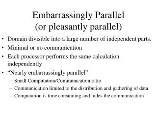
Embarrassingly Parallel Computations Chapter 3. Embarrassingly Parallel Computations. A computation that can obviously be divided into a number of completely independent parts, each of which can be executed by a separate process.

E N D
Embarrassingly Parallel Computations Chapter 3
Embarrassingly Parallel Computations A computation that can obviously be divided into a number of completely independent parts, each of which can be executed by a separate process. No communication or very little communication between processes Each process can do its tasks without any interaction with others
Practical embarrassingly parallel computation (static process creation / master-slave approach)
Embarrassingly Parallel Computations • Examples • Low level image processing • Many of such operations only involve local data with very limited if any communication between areas of interest. • Mandelbrot set • Monte Carlo Calculations
Some geometrical operations Shifting Object shifted by Dxin the x-dimension and Dyin the y-dimension: x¢ = x + Dx y¢ = y + Dy where x and y are the original and x¢ and y¢ are the new coordinates. Scaling Object scaled by a factor Sxin x-direction and Syin y-direction: x¢ = xSx y¢ = ySy Rotation Object rotated through an angle q about the origin of the coordinate system: x¢ = x cosq + y sinq y¢ = -x sinq + y cosq
Partitioning into regions for individual processes Square region for each process (can also use strips)
Mandelbrot Set What is the Mandelbrot set? Set of all complex numbers c for which sequence defined by the following iterationremains bounded: z(0) = c, z(n+1) = z(n)*z(n) + c, n=0,1,2, ... This means that there is a number B such that the absolute value of all iterates z(n) never gets larger than B.
Sequential routine computing value of one point • structure complex { • float real; • float imag; • }; • intcal_pixel(complex c) • { int count, max; • complex z; • float temp, lengthsq; • max = 256; • z.real = 0; z.imag = 0; • count = 0; /* number of iterations */ • do { • temp = z.real * z.real - z.imag * z.imag + c.real; • z.imag = 2 * z.real * z.imag + c.imag; • z.real = temp; • lengthsq = z.real * z.real + z.imag * z.imag; • count++; • } while ((lengthsq < 4.0) && (count < max)); • return count; • }
Parallelizing Mandelbrot Set Computation Static Task Assignment Simply divide the region into fixed number of parts, each computed by a separate processor. Disadvantage: Different regions may require different numbers of iterations and time. Dynamic Task Assignment
Monte Carlo Methods • Another embarrassingly parallel computation • Example: • calculate πusing the ratio: • Randomly choose points within the square • Count the points that lie within the circle • Given a sufficient number of randomly selected samples • fraction of points within the circle will be: π /4
Example of Monte Carlo Method Area = D2
Computing an Integral Use random values of x to compute f(x) and sum values of f(x): where xiare randomly generated values of x between x1 and x2. Monte Carlo method is very useful if the function cannot be integrated numerically (maybe having a large number of variables)
Example: Sequential Code sum = 0; for (i = 0; i < N; i++) { /* N random samples */ xr = rand_v(x1, x2); /* generate next random value */ sum = sum + xr * xr - 3 * xr; /* compute f(xr) */ } area = (sum / N) * (x2 - x1); Routine rand_v(x1, x2) returns a pseudorandom number between x1 and x2
Values for a "good" generator: a=16807, m=231-1 (a prime number), c=0 This generates a repeating sequence of (231- 2) different numbers.
A Parallel Formulation xi+1 = (axi + c) mod m xi+k = (Axi+ C) mod m A and C above can be derived by computing xi+1=f(xi) , xi+2=f(f(xi)), ... xi+k=f(f(f(…f(xi)))) and using the following properties: • (A+B) mod M = [(A mod M) + (B mod M)] mod M • [ X(A mod M) ] mod M = (X.A mod M) • X(A + B) mod M = (X.A + X.B) mod M = [(X.A mod M) + (X.B mod M)] mod M • [ X( (A+B) mod M) ] mod M = (X.A + X.B) mod M