Download
1 / 14
150 likes | 267 Views
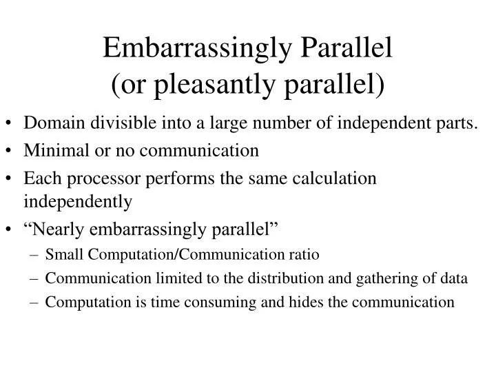
Embarrassingly Parallel (or pleasantly parallel). Domain divisible into a large number of independent parts. Minimal or no communication Each processor performs the same calculation independently “Nearly embarrassingly parallel” Small Computation/Communication ratio

E N D
Embarrassingly Parallel (or pleasantly parallel) • Domain divisible into a large number of independent parts. • Minimal or no communication • Each processor performs the same calculation independently • “Nearly embarrassingly parallel” • Small Computation/Communication ratio • Communication limited to the distribution and gathering of data • Computation is time consuming and hides the communication
Embarrassingly Parallel Examples P0 P1 P2 Embarrassingly Parallel Application Send Data P0 P1 P2 P3 Receive Data Nearly Embarrassingly Parallel Application
Low Level Image Processing • Storage • A two dimensional array of pixels. • One bit, one byte, or three bytes may represent pixels • Operations may only involve local data • Image Applications • Shifting (newX=x+delta; newY=y+delta) • Scaling (newX = x*scale; newY = y*scale) • Rotate(newX=x cosF+y sinF; newY=-xsinF+ysinF) • ClipnewX = x if minx<=x< maxx; 0 otherwisenewY = y if miny<=y<=maxy; 0 otherwise • Other Applications • Smoothing, Edge Detection, Pattern Matching
Process Partitioning 1024 128 768 P21 128 Partitioning might assign groups of rows or columns to processors
Image Shifting Application(See code on Page 84) • Master • Send starting row number to slaves • Initialize a new array to hold shifted image • FOR each message received • Update new bit map coordinates • Slave • Receive starting row • Compute translated coordinates and transmit them back to the master • Questions • Where is the initial image? • What happens if a remote processor fails? • How does the master decide how much to assign to each processor? • Is the load balanced (all processors working equally)? • Is the initial transmission of the row numbers needed?
Analysis Program on Page 84 • Computation • Host: 3 * rows * cols, Slave: 2 * rows * cols / (P-1) • Communication (tcomm= tstartup + m*tdata) • Host: (tstartup + tdata) * (P-1) + rows * columns * (tstartup + 4 * tdata) • Slaves: (tstartup+ tdata) + rows * columns/(P-1)*(tstartup+ 4 * tdata) • Total • Ts = 4 * rows * cols • Tp = 3 * rows*cols + (tstartup + tdata) * (P-1) + rows*cols * (tstartup+4 * tdata) = 3 * rows*cols + 2*(P-1) + 5*rows*cols = 8*rows*cols+2*(P-1) • S(p) < ½ • Computation ratio = tcomp/tcomm = (3*rows/cols)/(5*rows*cols+2*(p-1)) ≈ 3/5 • Questions • Can the transmission of the rows be done in parallel? • How is it possible to reduce the communication cost? • Is this an Amdahl or a Gustafson application?
Mandelbrot Set • The Mandelbrot Set is a set of complex plane points that are iterated • using a prescribed function over a bounded area: • The iteration stops when the function value reaches a limit • The iteration stops when the iteration count reaches a limit • Each point gets a color according to the final iteration count • Complex numbers • a+bi where i = (-1)1/2 • Complex plane • horizontal axis: real values • Vertical axis: imaginary values.
Pseudo code FOR each point c = cx+icy in a bounded area SET z = zreal + i*zimaginary = 0 + i0 SET iterations = 0 DO SET z = f(z, c) SET value = (zreal2 + zimaginary2)1/2 iterations++ WHILE value<limit and iterations<max point = cx and cy scaled to the display picture[point] = color[iterations] Notes: • Set each point’s color based on its final iteration count • Some points converge quickly; others slowly, and others not at all • The non converging points (exceeding the maximum iterations) are said to lie in the Mandelbrot Set (black on the previous slide) • A common Mandelbrot function is z = z2 + c
Scaling and Zooming • Display range of points • From cmin = xmin + iymin to cmax = xmax + iymax • Display range of pixels • From the pixel at (0,0) to the pixel at (width, height) • Pseudo code For pixelx = 0 to width For pixely= 0 to height cx = xmin + pixelx * (xmax – xmin)/width cy = ymin + pixely * (xmax – xmin)/height color = mandelbrot(cx, cy) picture[pixelx][pixely] = color
Parallel Implementation Static and Dynamic load balancing approaches shown in chapter 3 • Load-balancing • Algorithms used to avoid processors from becoming idle • Note: Does NOT mean that every processor has the same work load • Static Approach • The load is partitioned once at the start of the run • Mandelbrot: assign each processor a group of rows • Deficiencies of book approach • Separate messages per coordinate • No accounting for processes that fail • Dynamic Approach • The load is partitioned during the run • Mandelbrot: Slaves ask for work when they complete a section • Improvements from book approach • Ask for work before completion (double buffering) • Question: How does the program terminate?
Analysis of Static Approach • Assumptions (Different from the text) • Slaves send a row at a time • Assume display time is equal to computation time • tstartup and tdata = 1 • Master • Computation: height*width • Communication: height*(tstartup + width*tdata) ≈ height*width • Slaves • Computation: avgIterations * height/(P-1) * width • Communication: height/(P-1)*(tstartup+width*tdata) ≈height*width/P-1 • Speed-up • S(p) ≈ 2 * height * width * avgIterations • / (avgIterations*height*width/(P-1)+height*width/(P-1))≈ P-1 • Computation/communication ratio • 2 * height * width * avgIterations / (height * (tstartup + width*tdata))≈ avgIterations
Monte Carlo Methods Section 3.2.3 of Text • Pseudo-code (Throw darts to converge at a solution) • Compute definite integralWhile more iterations needed pick a point Evaluate a function Add to the answerCompute average • Calculation of PIWhile more iterations needed Randomly pick a point If point is in circle within++Compute PI = 4 * within / iterations • Parallel Implementation • Need a parallel pseudo random generator (See notes below) • Minimal communication requirements • Note: We can also use the upper right quadrant 1/N ∑1N f(pick.x) (xmax – xmin)
Computation of PI ∫(1-x2)1/2dx = π; -1<=x<=1 ∫(1-x2)1/2dx = π/4; 0<=x<=1 Within if (point.x2 + point.y2) ≤ 1 Total points/Points within = Total Area/Area in shape • Questions: • How to handle the boundary condition? • What is the best accuracy that we can achieve?
Parallel Random Number Generator • Numbers of a pseudo random sequence are: • Uniformly, large period, repeatable, statistically independent • Each processor must generate a unique sequence • Accuracy depends upon random sequence precision • Sequential linear generator (a and m are prime; c=0) • Xi+1 = (axi +c) mod m (ex: a=16807, m=231 – 1, c=0) • Many other generators are possible • Parallel linear generator with unique sequences • Xi+k = (Axi + C) mod m • A=aP, C=c (aP +aP-1 + …+a1 +a0) x1 x2 xP-1 xP-1 xP xP+1 x2P-2 x2P-1 Parallel Random Sequence