Download
1 / 7
70 likes | 167 Views
Transfer function model. Y(t) = + u a(t-u) X(u) + (t) dZ Y ( ) = A( ) dZ X ( ) + dZ ( ) Y(t) = exp{it } dZ Y ( ) Gas furnace data - Box & Jenkins Sampling interval 9 sec., observations for 296 pairs of data points

E N D
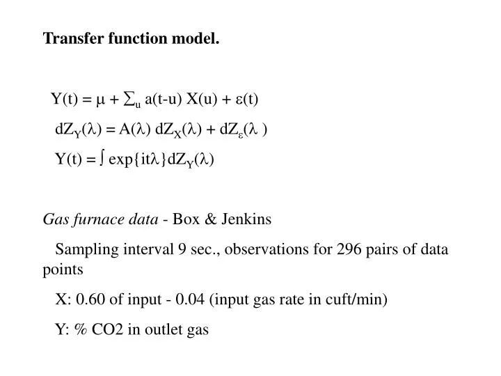
Transfer function model. Y(t) = + u a(t-u) X(u) + (t) dZY() = A() dZX() + dZ( ) Y(t) = exp{it}dZY() Gas furnace data - Box & Jenkins Sampling interval 9 sec., observations for 296 pairs of data points X: 0.60 of input - 0.04 (input gas rate in cuft/min) Y: % CO2 in outlet gas
Time side inference. Comparing alternate models. Supose there are J AICj = -2 log L(Ĝj ) + 2 sj sj is the number of paremeters in Gj There is also BICj = -2 log L(Ĝj ) + sj log nj Fundamental contributions of statistics