Download
1 / 27
270 likes | 425 Views
17 dicembre 2003. Luca Bortolussi. SUFFIX TREES. From exact to approximate string matching. An introduction to string matching. String matching is an important branch of algorithmica, and it has applications in many fields, as: Text searching Molecular biology Data compression and so on….

E N D
17 dicembre 2003 Luca Bortolussi SUFFIX TREES From exact to approximate string matching.
An introduction to string matching String matching is an important branch of algorithmica, and it has applications in many fields, as: • Text searching • Molecular biology • Data compression • and so on…
Exact String matching: a brief history • Naive algorithm • Knuth-Morris-Pratt (1977) • Boyer-Moore (1977) Suffix Trees: Weiner (1973), McCreight (1978), Ukkonen (1995)
Suffix Trees Definition: A suffix tree for a string T of length m is a rooted tree such that: • It has exactly m leafs, numbered from 1 to m; • Every edge has a label, which is a substring of T; • Every internal node has at least two children; • Labels of two edges starting at an internal node do not start with the same character; • The label of the path from the root to a leaf numbered I is the suffix of T starting at position i, i.e. T[i..m]
ab cbab# # 6 4 b bcbab# # ab# 7 1 5 cbab# bcbab# 3 2 Suffix Trees - II abbcbab#
ab cbab# # 6 4 b bcbab# # ab# 7 1 5 cbab# bcbab# 3 2 Suffix Trees – searching a pattern abbcbab# Pattern: bcb
Suffix Trees – naive construction abbcbab# ab cbab# # 6 4 b abbcbab# bbcbab# bcbab# # ab# 7 1 5 cbab# bcbab# 3 2
Suffix Trees – Ukkonen Algorithm Ukkonen algorithm was published in 1995, and it is the fastest and well performing algorithm for building a suffix tree in linear time. The basic idea is constructing iteratively the implicit suffix trees for S[1..i] in the following way: Construct tree I1 For i= 1 to m-1 // phase i+1 for j = 1 to i+1 // extension j find the end of the path from the root with label S[j…i] in the current tree. Extend the path adding character S(i+1), so that S[j…i+1] is in the tree. • The extension will follow one of the next three rules, being b= S[j..i]: • b ends at a leaf. Add S(i+1) at the end of the label of the path to the leaf • There’s one path continuing from the end of b, but none starting with S(i+1). Add a node at the end of b and a path stating from the new node with label S(i+1), terminating in a leaf with number j. • There’s one path from the end of b starting with S(i+1). In this case do nothing.
ab cbab# # 6 4 b bcbab# # ab# 7 1 5 cbab# bcbab# 3 2 Suffix Trees – Ukkonen Algorithm - II The main idea to speed up the construction of the tree is the concept of suffix link. Suffix links are pointers from a node v with path label xa to a node s(v) with path label a (a is a string and x a character). The interesting feature of suffix trees is that every internal node, except the root, has a suffix link towards another node. v S(v) abbcbab# Suffix link
Suffix Trees – Ukkonen Algorithm - III With suffix links, we can speed up the construction of the ST a xa g g b = ag In addition, every node can be crossed in costant time, just keeping track of the label’s length of every single edge. This can be done because no two edges exiting from a node can start with the same character, hence a single comparison is needed to decide which path must be taken. Anyway, using suffix links, complexity is still quadratic.
Suffix Trees – Ukkonen Algorithm - IV Storing the path labels explicitly will cost a quadratic space. Anyway, each edge need only costant space, i.e. two pointers, one to the beginning and one to the end of the substring it has as label. • To complete the speed up of the algorithm, we need the following observations: • Once a leaf is created, it will remain forever a leaf. • Once in a phase rule 3 is used, all succeccive extensions make use of it, hence we can ignore them. • If in phase i the rule 1 and 2 are applied in the first ji moves, in phase i+1 the first ji extensions can be made in costant time, simply adding the character S(i+2) at the end of the paths to the first ji leafs (we will use a global variable e do do this). Hence the extensions will be computed explicitly from ji+1, reducing their global number to 2m.
c$ ab c# (1,4) (2,4) b (2,2) bc$ abc# (1,1) c$ bc$ (2,1) (1,3) (2,3) (1,2) Generalized Suffix Trees A generalized suffix tree is simply a ST for a set of strings, each one ending with a different marker. The leafs have two numbers, one identifiing the string and the other identifiing the position inside the string. S1 = abbc$ S2 = babc#
Longest common substring Let S1 and S2 be two string over the same alphabeth. The Longest Common Substring problem is to find the longest substring of S1 that is also a substring of S2. Knuth in 1970 conjectured that this problem was Q(n2) Building a generalized suffix tree for S1 and S2, to solve the problem one has to identify the nodes which belong to both suffix trees of S1 and S2 and choose the one with greatest string depth (length of the path label from the root to itself). All these operations cost O(n).
Longest Common Extension A problem that can be solved linearly using suffix trees is the Longest Common Extension problem, that is, for every couple of indexes (i,j), finding the length of the longest substring of T starting at position i that matches a substring of P starting at position j. It can be solved in O(n+m) time, building a generalized suffix tree for T and P, and finding, for every leaf i of T and j of P, their lowest common ancestor in the tree (it can be done in costant time after preprocessing the tree).
Hamming and Edit Distances Hamming Distance: two strings of the same length are aligned and the distance is the number of mismatches between them. abbcdbaabbc H = 6 abbdcbbbaac Edit Distance: it is the minimum number of insertions, deletions and substitutions needed to trasform a string into another. abbcdbaabbc abbcdbaabbc E = 3 cbcdbaabc abbcdbaabbc
The k - mismatches problem We have a text T and a pattern P, and we want to find occurences of P in T, allowing a maximum of k mismatches, i.e. we want to find all the substring T’ of T such that H(P,T’) ≤ k. We can use suffix trees, but they do not perfome well anymore: the algorithm scans all the paths to leafs, keeping track of errors, and abandons the path if this number becomes greater that k. The algorithm is fastened using the longest common extensions. For every suffix of T, the pieces of agreement between the suffix and P are matched together until P is exausted or the errors overcome k. Every piece is found in costant time. The complexity of the resulting algorithm is O(k|T|). aaacaabaaaaa…. c An occurence is found in position 2 of T, with one error. aabaab b
Inexact Matching • In biology, inexact matching is very important: • Similarity in DNA sequences implies often that they have the same biological function (viceversa is not true); • Mutations and error transcription make exact comparison not very useful. • There are a lot of algorithms that deal with inexact matching (with respect to edit distance), and they are mainly based on dynamic programming or on automata. Suffix trees are used as a secondary tools in some of them, because their structure is inadapt to deal with insertions and deletions, and even with substitutions. • The main efforts are spend in fastening the average behaviour of algorithms, and this is justified because of the fact that random sequences often fall in these cases (and DNA sequences have an high degree of randomness).
Dynamic Programming We aim to compute edit distance (global alignements) between two string S and T • The main idea is computing the edit distance between any of the prefixes of S and T. Let D(i,j) be this distance. Of course, the edit distance between S and T is D(n,m), where n=|P| and m=|T|. • The following properties hold: • D(i,0) = i, D(0,j) = j; • D(i,j) = min { D(i,j-1) + 1, D(i-1,j) + 1, D(i-1,j-1) + t(i,j) }. Hence in O(mn) time we can compute a matrix which encodes not only the edit distance, bu also the way to trasform a string into another (just keeping track, by means of pointers, of which elements realize the minimum)
Dynamic Programming II C A S E 1 2 3 4 0 0 1 2 3 4 0 A 1 1 1 2 3 1 R 2 2 2 2 3 2 E 3 3 3 3 2 3
Non-Deterministic Automata To recognize the approximate occurences of a pattern P in a text T, we can build a non-deterministic automaton for P, and run it with T as input. This leads to faster algorithms for the search, but the problem is building the automaton. C A S E S S S S S S S S S e e e e C A S E S S S S S S S S S e e e e C A S E
Longest Common Subsequence The Longest Common Subsequence between two strings S1 and S2 is the greater number of characters of S1 that can be aligned to S2. It is a global alignement problem, which is obviously connected with edit distance. Anyway, often it is modelled with a scoring scheme, which gives a positive score to matches and a negative one to mismatches, insertions and substitutions. So the best global alignement is the one which maximizes the total score. Clearly, given the best global alignement, the number of matches is the longest common subsequence solution. a b b c d a b b a a b _ c b a b _ a
The k – differences problem This problem is to find all the occurences of a pattern P in a text T, allowing a maximum number of k insertions, deletions or substitutions. The Landau-Vishkin algorithm solves it in O(k|T|) time, and implements an hybrid dynamic programming tecnique, which uses suffix trees to solve a subproblem. The algorithm looks for paths in the dynamic programming matrix (which start in the upper row), in particular for d-paths, which are paths that specify exactly d mismatches and spaces. Some of these paths are computed, for d ≤ k, and the ones that reach the bottom row correspond to approximate occurences of P in T, with exactly d mismatches or spaces.
Inexact Matching, a new approach Suffix trees work very well for exact matching, but they fail when we admit errors in the matching process. This happens because, the only way to find approximate occurences of a pattern, when we search it in a suffix tree, is to walk down every path, keeping track of errors and discarding the paths which overcome the tolerance level previously chosen. A different approach may be that of defining a different data structure, though similar to suffix trees, which encodes in some way a concept of distance, in particular the Hamming Distance. A possible way is to shift from alphabeth A to alphabet Ak, encoding the distance in a relation between letters: two letters are said to be “equivalent” if and only if their Hamming distance is less than a threshold d.
Equivalence between letters Let’s show and example of this idea of equivalence, with A = {0,1} andk = 3. So, we can build the following table for A3: If the distance between two letters is less or equal than 1, we define them equivalent. For example ab, bd, but NOT(ad).
Bundled Suffix Trees Given this equivalence relation (which is not transitive), we want to incorporate it in a tree structure. For simplicity, we assume that the tree for the sequence S is the smallest tree which contains, for every substring of S, all the exact paths and all the equivalent paths that can be found in S. For “historical reasons”, we will call it a Bundled Suffix Tree. • Definition: A bundled suffix tree B for a string S of length m is a rooted tree such that: • It has exactly m leafs, numbered from 1 to m; • Every edge has a label, which is a substring of S; • Every node has a set of labels, which is a subset of {1,2,..,m,s}; • The tree obtained deleting all nodes which do not has s as label is the suffix tree for S; • For every substring P of S, the subtree of B rooted at the end of the path labeled with P has node labels which union (discarding s) gives all the starting positions of substrings of S equivalent to P; • In every path from the root to a leaf no two nodes can be labelled with the same number.
a b d c a d a # # c b b d bcd a a# c # bcd d a a # # Bundled Suffix Trees - II abbcda# s s,6 6 s 1,4 s,5 2 s 5,3 5 2 3 1 s,1 s,4 3 4 2 1 s,3 s,2
Open Problems 1. Does BST work well for Hamming distance? (they seem to need a distributed distance). 2. How can BST be used to manage approximate searching using edit distance? At what price? 3. Which is the average number of “red” nodes expected? Is it linear or does it grows quadratically? 4. Is there a linear algorithm for building BST? 5. Does BST manage to improve existant algorithms, or the interest is just theoretical?