Normal Distribution

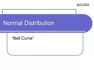
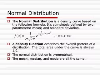
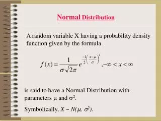
1. Normal Distribution • The normal distribution was first introduced by the French mathematician La Place (1749-1827). • It is highly useful in the field of statistics. The graph of this distribution is called normal curve or bell-shaped curve. • In normal distribution, observations are more clusters around the mean. Normally almost half the observations lie above and half below the mean and all observations are symmetrically distributed on each side of the mean. • The normal distribution is symmetrical around a single peak so that mean median and mode will coincide. It is such a well-defined and simple shape, a great deal is known about it. The mean and standard deviation are the only two values we need to know o be able to describe a normal curve completely.

2. Normal Distribution

3. Normal Distribution • Characteristics : • The curve is symmetrical • It is a bell shaped curve. • Maximum values at the center and decrease to zero symmetrically on each side • Mean, median and mode coincide • Mean = Median = Mode • It is determined by mean and standard deviation. • Mean1SD limits, includes - 68% of all observations • Mean  2SD - ,, ,, - 95% ,, ,, • Mean  3SD - ,, ,, - 99% ,, ,,

4. Normal Distribution • Almost all statistical tests (t-test, ANOVA etc) assume normal distributions. These tests work very well even if the distribution is only approximately normally distributed. • Some tests (Mann-whitney U test, Wilcoxon W test etc) work well even with very wide deviations from normality.

5. One Two Three or more Mean±SD t-test Unpaired t-test  Paired t-test Median (Range) Non-parametric t-test (or Rank Test)  The Mann-Whitney U test  The Wilcoxon Matched-Pairs Signed- Ranks Test • The Kruskal-Wallis One-way ANOVA by Ranks • The Friedman’s Test Normal Distribution Group Distribution is normal Distribution is not normal (Parametric tests) (Nonparametric tests) • One Way ANOVA • The Repeated Measures ANOVA Relationship between two variables •  The Correlation Coefficient •  Simple Linear Regression The Spearman Rank Correlation Coefficient  Nonparametric Regression Analysis

6. Tests of Significance (testing hypothesis) Definition: A significance test is a statistical test (mathematical methods) that estimates that the observed difference between two or more groups is due to chance or not. • Statistical tests (such as t-test, F-ratio, and chi-square) ultimately lead to a p-value which is used to make a statement/conclusion about the statistical significance of the results that is for example: a difference between means of experimental and control groups are statistically significantly differ or not.

7. Tests of Significance • The concept of statistical significance is based on the assumption that events which occur rarely by chance are "significant". Traditionally, events which occur less than 5 out of 100 (or p–value <0.05) are said to be statistically significant. • Methods of determining the significance of difference (test of significance) are used to draw inference and conclusions. • Based on distribution (whether normal distribution or not) test of significance are two types. • (1)Parametric test:t-test, ANOVA etc • (2)Nonparametric test: Mannwhitney-U test, Wilcoxon-W test, test etc

8. Hypothesis • A hypothesis is an assumption to be tested. • Hypothesis tests are widely used for making decisions i.e. very often we make decision about population on the basis of sample information • For example: we may decide on the basis of sample data whether a new medicine is really effective in curing a disease. • Two types of hypothesis: Null hypothesis: H0 and alternative hypothesis: H1 • Null hypothesis (Hypothesis of indifference): A hypothesis which states that there is no difference between two samples. The null hypothesis is often the ‘’straw man’’ that we wish to reject. Philosophers of science tell us that ‘we never prove things conclusively; we can only disprove theories’. • Alternative hypothesis:is the opposite of null hypothesis (or any hypothesis other than null hypothesis), i.e., there is difference between the two samples.

9. Stages in performing a test of significance • The first step in hypothesis testing is to establish the hypothesis to be tested. State the null hypothesis of no difference and the alternative before test of significant, eg. Vit A and D makes no difference in growth or alternatively they play a positive or significant role in promoting growth. • Choose the desired level of significance, denoted by ‘a’ (usually a = 0.05 or 0.01). • Choose a appropriate test of statistics (eg t test, ANOVA, chi- square etc) to test the null hypothesis.

10. Stages in performing a test of significance (continuation) • Determine p value, the probability of occurrence of the estimate by chance, i.e., accept or reject the null hypothesis. If p is less than a certain amount (by convention 5% or o.o5), we consider null hypothesis to be unlikely and we reject it. • Draw conclusion on the basis of p value, either accepting null hypothesis or rejecting it, i.e., decide whether the difference observed is due to chance or play of some external factors on the sample under study. • For example: H0: there is no association between personal hygiene and occurrence of diarrhoea. After doing test of significance (chi-square test) it was figured out that the calculated value (say 11.18) was more than the tabulated value (say 3.84) indicating that p<0.05; so the conclusion will be null hypothesis is rejected and alternative hypothesis is accepted, i.e. there is association between personal hygiene and occurrence of diarrhea.

11. P value • P valuestands for probabilityof by chance. • P value is quoted widely in the medical literature. They are scattered through articles in medical research, clinical trials, epidemiological studies, sample surveys and laboratory work. • P values are standard device for reporting quantitative results in research where variability plays a large role. Statement like “blood glucose level of type 1 diabetes is significantly (p<0.05) higher than type 2 diabetes.

12. P value • P value is used toassess the degree of dissimilaritybetween two or more groups of observations. It indicates the probability of occurrence of the difference by chance. • P value measures the chance of dissimilarity between two or more set of measurements or between one set ofmeasurements and a standard. • P = 0.05 means - the difference between two different groups is significant at the level of 5%. • If p<0.05, the test hypothesis is rejected and p>0.05 it is accepted.

13. P value “P valueis the probability of being wrong when asserting that a true difference exist between the different treatment groups.” • If p<0.05, the result is regarded as statistically significant • If p<0.01, ,, ,, ,, moderately ,, • If p<0.001 highly ,, • If p> 0.10, the result is regarded as no statistically significant

14. Significance of Difference in Two Means If the statistics observed in the two means, say and , the question refer to whether they differ significantly or the difference found is due to chance error of sampling. If on the basis of a test, we find that the difference is too large to attribute to chance errors, we will conclude that the sample means are unequal or statistically significant different.

15. Significance of Difference in Two Means Depending on the size of sample the test of significance of difference in two means are two types: • z-test (for large samples, >30) • t-test (for small samples).

16. Z-test (for large samples, >30) To test the difference between two population means, the test statistic is Where and are variances of two samples Example: The haemoglobin (Hb) level of children was measured in 143 girls and 127 boys. The results were as follows: Number (n) Mean (Hb%) SD Girls 143 11.2 1.4 Boys 127 11.0 1.3

17. Z-test (for large samples, >30) The test procedure is as follows: 1. State the null hypothesis: mean Hb is same in girls as well as in boys. 2.Find z value using mean difference (11.2 – 11.0 = 0.2), , , n1 and n2. 3. Refer the z value to find the probability of the observed difference by chance (p value) form table. If p-value is large, we can not reject the null hypothesis, so we have to conclude that these data give no evidence of a real sex difference.

18. Z-test (for large samples, >30) Here n1 = 143, =11.2, s1 = 1.4 n2 = 127, = 11.0, s2 = 1.3 Therefore, = 1.22 Since z<1.96, p>0.05, the difference is not statistically significant, i.e. it could easily have occurred by chance.

19. t-test (for small samples, <30) 2 types of t-test 1. Unpaired t-test (two independent samples) 2. Paired t-test (single sample correlated observations) Unpaired t-test: Criteria 1. Data are quantitative 2. Normal distribution. 3. Observations are independent of each other. 4. Sample size is less than 30 t test can be used in two types of cases: the case in which variances are equal, i.e., 12 = 22 b. the case in which variances are not equal, i.e., 12 = 22

20. t-test (for small samples, <30) Unpaired t-test (in case of equal variance ) When population variances (though unknown) can be assumed equal then the appropriate test statistic is Student’s t defined by Where With degree of freedom = n1+n2-2 Degree of freedom = freedom of choice

21. Unpaired t-test (in case of equal variance): Example Two different types of drugs A and B were tried on certain patients for increasing weight, 5 persons given drug A and 7 persons given drug B. Do the drugs differ significantly with regard to their effect in increasing weight? Null hypothesis: H0: there is no difference in the efficacy of the two drugs. d.f. = n1+n2-2 = 5+7-2 = 10

22. Unpaired t-test (in case of equal variance): Example Interpretation: The calculated value (0.5) of ‘t’ is less than the table value (1.81), ie, p>0.05. Therefore, our hypothesis is accepted. Hence, we conclude that there is no significant difference in the efficacy of the two drugs in case of increasing weight.

23. t-test (for small samples, <30) Unpaired t-test (in case of unequal variance ) Sometime it is not reasonable to assume equality of the population variance and hence we cannot apply normal test as well because of the smallness of the sample size. In such case, we apply t-test, defined as follows: Where degree of freedom is

24. t-test (for small samples, <30) Paired t-test: Paired t-test is applied for paired data. Typically paired data refers to repeated or multiple measurements on the same subjects. Application: Paired t-test is used to compare difference between means of paired samples, e.g., cross over trials, different time in the same group (‘’before-after studies’’ and ‘’twin studies’’) Example:To compare a measurement of the level of pain before and after administration of an analgesic drug. Criteria: 1. The data are quantitative 2. Normal distribution 3. paired data

25. t-test (for small samples, <30) Paired t –test is defined by Where = mean of difference, SE ( ) = SE of the mean difference.

26. Paired t-test (Example) Problem:Antihypertensive effect of a drug was tested on 15 individuals. The recording of diastolic blood pressure are shown in the table Interpret: The data justifies application of paired t-test. Step 1: Null hypothesis: There is no difference in the diastolic B.P. before and after the drug treatment. The observed difference is due to sampling variation. Alternative hypothesis: The observed difference is due to drug. Step 2: Calculate mean difference in the pairs. Step 3: Calculate standard deviation (SD) and standard error Step 4: Calculate t: Step 5: calculate degree of freedom (df): [df = n-1] Step 6: find out probability (p value) Step 7: Interpretation.

27. Paired t-test (Example) Problem: Antihypertensive effect of a drug was tested on 15 individuals. The recording of diastolic blood pressure are shown in the table

28. Paired t-test (Example) d.f. = n – 1 = 15 – 1 = 14 Step 7: Interpret: The table value of t at 5% level of significance for 14 d.f. is 1.76. Computed value is 4.89. Since the computed value (4.89) is much more higher than the table value (1.76) at 5%, ie, the p value is less than 0.05. Hence, null hypothesis is rejected, alternative hypothesis is accepted, and the difference in before & after values is considered statistically significant.

29. Sampling errors: Type I & Type II error Sampling error: Sampling error are errors due to chance and concern incorrect rejection or acceptance of a null hypothesis. It depends on selection of level of hypothesis. Type I error: A Type I error occurs when the null hypothesis is rejected when, in fact, it is true. Type II error: A Type II error occurs when the null hypothesis is not rejected when it is false.

30. Why not just use the t-test to compare more than 2 means? • The t-test tells us if the variation between two groups is "significant", • But how do we interpret significant variation among the means of 3 or more groups? Why not just do t-tests for all the pairs of means. • Multiple t-tests are not the answer because as the number of groups grows, the number of needed pair comparisons grows quickly. For 7 groups there are 21 pairs [No of paired to be tested = k(k-1)/2, k = no. of groups].

31. Why not just use the t-test to compare more than 2 means? • The difficulty here is that multiple significance testing (by t-test) gives a high probability of finding a significant difference just by chance. • When performing k multiple independent significance tests each at the a level, the probability of making at least one Type 1 error (rejecting the null hypothesis inappropriately) is1-(1-a)k. • For example, with k (pairs of comparisons)=10 and a(level of significance) = 0.05, there is a 40% chance of at least one of the ten tests being declared significant under the null hypothesis. So, when there is a significant result among the ten tests, there is 40% chance that something will turn out significant, ie, group-wise Type 1 error rate is actually 40% - a far cry from the 5% that may have thought it was.

32. Why not just use the t-test to compare more than 2 means? a = 1-(1-a)k. • ANOVA puts all the data into one number (F value) and gives us oneP for the null hypothesis and controlling type 1 error rate at no more than 5%.

33. ANOVA (Aanalysis of Variance) ANOVA or `F’ test used to analyze the variance for judging the significance of more than 2 means. ANOVA replace the multiple t- test with a single ‘F’ test. Hypothesis: All the groups have a common population mean or do the groups have equal means. The calculated value of F is compared with the table value of F for the given degree of freedom at a certain critical level. If the calculated value of F is greater than the table value of F, it indicates that the difference in sample means is significant or, in the other words the samples do not come from the same population. On the other hand, if the calculated value of F is less than the table value, the difference is not significant and hence could have arisen due to fluctuations of random sampling.

34. ANOVA -Calculation 1. Calculation of the variance between the groups: For calculating variance between groups, we take the sum of the square of the deviations of the means of the various groups from the grand grand mean and divide this sum by the degree of freedom. Steps: Calculate the mean of each group, eg. Calculate the grand mean Take the difference between the means of the various groups and grand mean. Square these deviations and obtain the sum which will give the sum of square between the groups and divide this by the degree of freedom (df = No. of groups – 1). N = number of groups

35. ANOVA -Calculation 2. Calculation of the variance within the groups: For calculating variance within the groups, we take the sum of the square of the deviations of various observations from the mean of the respective group and divide this sum by the degree of freedom (number of observation in each group). Steps: Calculate the mean of each group, eg. Take the deviations of the various observation from the means of the respective group. Square these deviations and obtain the sum which gives the sum of square within the groups and divide this by the degree of freedom (df = No of observation of each group – 1) Add all these variances and divide by the number of groups/variance. 3. Calculate the F-ratio:

36. ANOVA –Calculation (Alternative way) Variance is computed as the sum of squared deviations from the overall mean, divided by n-1 (sample size minus one, ie., degree of freedom). Thus given a certain n, the variance is a function of the sums of (deviation) squares, or SS for short. Calculation of degree of freedom (df): df for between groups = Number of groups minus one = column -1 = (c-1) df for within groups = Number of cases in each group minus one and added, (1st group – 1) + (2nd group – 1) + (3rd group – 1) = total number – column = (n-c) Df Sum of squares Mean sum of squares F (variance) (MS) Between groups(c – 1) SSB SSB / (c-1) Within groups(n – c ) SSW SSW / (n-c)

37. ANOVA - Exercise Problem: Three different treatment are given to 3 groups of patients with anemia. Increase in Hb% level was noted after one month and is given below. Find whether the difference in improvement in 3 groups is significant or not. N = 7+7+7= 21 = 23+40+90 = 153 = 11+16+24 = 51

38. df Sum of squares Mean sum of squares F (variance) Between groups2 (3-1) 12.28 6.14 Within groups18 [(7-1)+ (7-1)+ (7-1)] 16.86 0.94 6.53 ANOVA - Exercise • Steps: • 1. Calculation of total sum of squares (SST) (for all values) • 2. Calculation of ‘between’ sum of square (SSB) (ie, between group) • (T= Total) • 3. Calculation of ‘within’ sum of squares (SSW) (ie, within group) • SSw = SST – SSB = 29.14 - 12.28 = 16.86 (N= total numbers in all groups)

39. ANOVA - Excercise Df Sum of squares Mean sum of squares F Between groups 2 12.28 6.14 6.53 Within groups 18 16.86 0.94 Interpretation: F- value in the table at 2, 18 df (n1=2, n2=18) is 3.55 (at 5% significance level). Our calculated value is 6.53, which is more than table value (3.55). So it is significant

40. Multiple comparison methods Ordinary ANOVA compares all groups and confirms difference among the groups but it does not tell us which group differs from which others. Multiple comparison methods (eg Bonferroni, Dunnett, Duncan’s Tukey tests etc.) solve this problem and control over all type 1 error rate at no more than 5%.They are also known as post-hoc tests. We can find all the pair wise difference among the group means and test them individually for significance. Basically they adjust the p value for declaring statistical significance.

41. Bonferroni test It is based on the the t-statistic and thus can be considered a form of t-test. Bonferroni test uses the same criterion of setting the alpha error rate to the experiment-wise error rate (usually a = 0.05) divided by the total number of comparisons to control for Type I error when multiple comparisons are being made. Where, ab = 0.05 and k = number of comparisons = 10. So if we apply a significant level of 0.005 to each of the 10 tests/comparisons, there is now only a 5% chance that any of them will be declared significant under null hypothesis. This modification is referred to as the Bonferroni correction.

42. Bonferroni test The t test for treatment means following analysis of variance is given by = the within-treatments variance = the mean of treatment group number i = the number of individuals in treatment group number i

43. Bonferroni test • For small number of comparisons (say up to 5) its use is reasonable, but for large numbers it is highly conservative, leading to p values that are too high. It is minor concern when compare only few groups (<5) but is a major problem when you have many groups. • Therefore, Bonferroni is not used with more than 5 groups. • For large number of comparisons (>5 pairs) Duncan’s or Tukey multiple range test is recommended. They are less conservative than the Bonferroni method.

44. Dunnett’s Test: Multiple comparisons against a single control group is Dunnett’s test. This test is suitable for small number of comparisons. It is used when the researcher wishes to compare each treatment group mean with the mean of the control group.

45. Tukey test:  The Tukey method is preferred when the number of groups is large as it is a very conservative pairwise comparison test, and researchers prefer to be conservative when the large number of groups threatens to inflate Type I errors. Some recommend it only when all pairwise comparisons are being tested. The Tukey HSD test is based on the q-statistic (the Studentized range distribution) and is limited to pairwise comparisons.