Download
1 / 69
690 likes | 843 Views
Transfer Learning for Image Classification. Transfer Learning Approaches. Leverage data from related tasks to improve performance: Improve generalization. Reduce the run-time of evaluating a set of classifiers. Two Main Approaches: Learning Shared Hidden Representations.

E N D
Transfer Learning Approaches • Leverage data from related tasks to improve performance: • Improve generalization. • Reduce the run-time of evaluating a set of classifiers. • Two Main Approaches: • Learning Shared Hidden Representations. • Sharing Features.
Sharing Features: efficient boosting procedures for multiclass object detection Antonio Torralba Kevin Murphy William Freeman
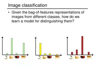
Snapshot of the idea • Goal: • Reduce the computational cost of multiclass object recognition • Improve generalization performance • Approach: • Make boosted classifiers share weak learners • Some Notation:
Training a single boosted classifier • Consider training a single boosted classifier: Candidate weak learners Weighted stumps Fit an additive model
Training a single boosted classifier Minimize the exponential loss Greedy Approach GentleBoosting
Standard Multiclass Case: No Sharing Additive model for each class Minimize the sum of exponential losses Each class has its own set of weak learners:
Multiclass Case: Sharing Features subset of classes correspondingadditive classifier classifier for the k class At iteration t add one weak learner to one of the additive models: Minimizethe sum of exponential losses Naiveapproach: Greedy Heuristic:
Sharing features for multiclass object detection Torralba, Murphy, Freeman. CVPR 2004
Sharing features shows sub-linear scaling of features with objects (for area under ROC = 0.9). Red: shared features Blue: independent features
How the features are shared across objects Basic features: Filter responses computed at different locations of the image
Uncovering Shared Structuresin Multiclass Classification Yonatan Amit Michael Fink Nathan Srebro Shimon Ullman
Structure Learning Framework Linear Classifiers Linear Transformations Class Parameters Structural Parameters • Find optimal parameters:
Multiclass Loss Function • Hinge Loss: • Maximal Hinge Loss:
Snapshot of the idea • Main Idea: Enforce Sharing by finding low rank parameter matrix W Transformation on x Transformation on w • Consider the m by d parameter matrix: • Can be factored: • Rows of theta form a basis
Low Rank Regularization Penalty • Rank of a d by m matrix is the smallest z, such that: • A regularization penalty designed to minimize the rank of W’ would tend to produce solutions where a few basis are shared by all classes. • Minimizing the rank would lead to a hard combinatorial problem • Instead use a trace norm penalty: eigen value of W’
Putting it all together No longer in the objective • For optimization they use a gradient based method that minimizes a smooth approximation of the objective
Transfer Learning for Image Classification via Sparse Joint Regularization Ariadna Quattoni Michael Collins Trevor Darrell
Training visual classifiers when a few examples are available • Problem: • Image classification from a few examples can be hard. • A good representation of images is crucial. • Solution: • We learn a good image representation using: unlabeled data + labeled data from related problems
Snapshot of the idea: • Use unlabeled dataset + kernel function to compute a new representation: • Complex features, high dimensional space • Some of them will be very discriminative (hopefully) • Most will be irrelevant • If we knew the relevant features we could learn from fewer examples. • Related problems may share relevant features. • We can use data from related problems to discover them !!
Semi-supervised learning Step 1: Learn representation Visual Representation Large dataset of unlabeled data Unsupervised learning Step 2: Train Classifier h-dimensional training set Small training set of labeled images Compute Train Classifier
Semi-supervised learning: • Raina et al. [ICML 2007] proposed an approach that learns a sparse set of high level features (i.e. linear combinations of the original features) from unlabeled data using a sparse coding technique. • Balcan et al. [ML 2004] proposed a representation based on computing kernel distances to unlabeled data points.
Learning visual representations using unlabeled dataonly • Unsupervised learning in data space • Good thing: • Lower dimensional representation preserves relevant statistics of the data sample. • Bad things: • The representation might still contain irrelevant features, i.e. features that are useless for classification.
Learning visual representations from unlabeled data + labeled data from related categories Step 1: Learn a representation Labeled images from related categories Large Dataset of unlabeled images Kernel Function Discriminative representation Select Discriminative Features of the New Representation Create New Representation
Our contribution • Main differences with previous approaches: • Our choice of joint regularization norm allows us to express the joint loss minimization as a linear program (i.e. no need for greedy approximations.) • While previous approaches build joint sparse classifiers on the feature space our method discovers discriminative features in a space derived using the unlabeled data and uses these discriminative features to solve future problems.
Overview of the method • Step I: Use the unlabeled data to compute a new representation space [Kernel SVD]. • Step II: Use the labeled data from related problems to discover discriminative features in the new space [Joint Sparse Regularization]. • Step III: Compute the new discriminative representation for the samples of the target problem. • Step IV: Train the target classifier using the representation of step III.
Step I: Compute a representation using the unlabeled data • Perform Kernel SVD on the Unlabeled Data. • A) Compute kernel matrix of unlabeled images: U K • B) Compute a projection matrix A by taking all the eigen vectors of K.
Step I: Compute a representation using the unlabeled data • C) Project labeled data from related problems to the new space: D • Notational shorthand:
Sidetrack • Another possible method for learning a representation from the unlabeled data would be to create a projection matrix Q by taking the h eigen vectors of A corresponding to the h largest eigenvalues. • We will call this approach the Low Rank Baseline • Our method differs significantly from the low rank approach in that we use training data from related problems to select discriminative features in the new space.
Step II: Discover relevant features by joint sparse approximation • A classifier is a function: where: is the input space, i.e. the representation learnt from unlabeled data. and is a binary label, in our application is going to be 1 if an image belongs to a particular topic and -1 otherwise. • A loss function:
Step II: Discover relevant features by joint sparse approximation • Consider learning a single sparse linear classifier (on the space learnt from the unlabeled data) of the form: • A sparse model will have only a few features with non-zero coefficients. • A natural choice for parameter estimation would be: L1 penalizes non-sparse solutions Classification error • Donoho [2004] has proven (in a regression setting) that the solution with smallest L1 norm is also the sparsest solution.
Step II: Discover relevant features by joint sparse approximation • Goal: Find a subset of features Rsuch that each problem in: can be well approximated by a sparse classifier whose non-zero coefficients correspond to features in R. • Solution : Regularized Joint loss minimization: penalizes solutions that utilize too many features Classification error on training set k
Step II: Discover relevant features by joint sparse approximation • How do we penalize solutions that use too many features? Coefficients for for feature 2 Coefficients for classifier 2 • Problem : not a proper norm, would lead to a hard combinatorial problem .
Step II: Discover relevant features by joint sparse approximation • Instead of using the #non-zero-rows pseudo-norm we will use a convex relaxation [Tropp 2006] • This norm combines: An L1 norm on the maximum absolute values of the coefficients promotes sparsity on max values. Use few features The L∞ norm on each row promotes non-sparsity on the rows Share features • The combination of the two norms results in a solution where only a few features are used but the features used will contribute in solving many classification problems.
Step II: Discover relevant features by joint sparse approximation • Using the L1- L∞ normwe can rewrite our objective function as: • For any convex loss this is a convex function, in particular when considering the hinge loss: the optimization problem can be expressed as a linear program.
Step II: Discover relevant features by joint sparse approximation • Linear program formulation ( hinge loss): • Max value constraints: and • Slack variables constraints: and
Step III: Compute the discriminative features representation • Define the set of relevant features to be: • Create a new representation by taking all the features in x’ corresponding to the indexes in R
Experiments: Dataset Reuters Dataset 10382 images, 108 topics . Predict 10 most frequent topics; (binary prediction) Data Partitions 3000 unlabeled images. 2382 images as testing data. 5000 images as source of supervised training data labeled training sets of sizes: 1, 5, 10 ,15…50. Training set with n positive examples and 2*n
Dataset SuperBowl [341] Danish Cartoons [178] Australian open [209] Trapped coal miners [196] Sharon [321] Golden globes [167] Grammys [170] Figure skating [146] Academy Awards [135] Iraq [ 125]
Baseline Representation • ‘Bag of words’ representation that combines: color, texture and raw local image information • Sampling: • Sample image patches on a fixed grid • For each image patch compute: • Color features based on HSV color histograms • Texture features based on mean responses of Gabor filters at different scales and orientations • Raw features, normalized pixel values • Create visual dictionary: for each feature type we do vector quantization and create a dictionary V of 2000 visual words.
Baseline representation • Compute baseline representation: • Sample image patches over a fix grid • For every feature type map each patch to its closest visual word in the corresponding dictionary. • The final representation is given by: where is the number of times that an image patch was mapped to the i-th color word
Setting • Step 1: Learn a representation using the unlabeled datataset and labeled datatasets from 9 topics. • Step 2: Train a classifier for the 10th held out topic using the learnt representation. • As evaluation we use the equal error rate averaged over the 10 topics.
Experiments • Three models, all linear SVMs • Baseline model (RFB): • Uses raw representation. • Low Rank baseline (LRB): • Uses as a representation: where Q is consists of the h highest eigenvectors of the matrix A computed in the first step of the algorithm • Sparse Transfer Model (SPT) • Uses Representation computed by our algorithm • For both LRB and SPT we used and RBF kernel when computing the Representation from unlabeled data.
Results: Mean Equal Error rate per topic for classifiers trained with five positive examples; for the RFB model and the SPT model. SuperBowl; GG: Golden Globes; DC: Danish Cartoons; Gr: Grammys; AO: Australian Open; Sh:Sharon; FS: Figure Skating; AA: Academy Awards; Ir: Iraq.
Conclusion • Summary: • We described a method for learning discriminative sparse image representations from unlabeled images + images from related tasks. • The method is based on learning a representation from the unlabeled data and performing joint sparse approximation on the data from related tasks to find a subset of discriminative features. • The induced representation improves performance when learning with very few examples.