Download
1 / 29
1.94k likes | 4.27k Views
Inter-observer variation can be measured in any situation in which two or more independent observers are evaluating the same thing Kappa is intended to give the reader a quantitative measure of the magnitude of agreement between observers .

E N D
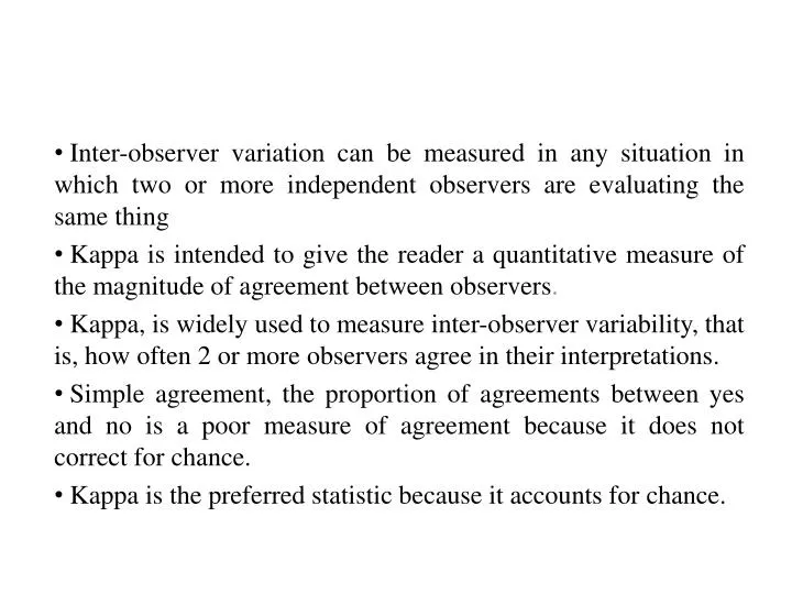
Inter-observer variation can be measured in any situation in which two or more independent observers are evaluating the same thing Kappa is intended to give the reader a quantitative measure of the magnitude of agreement between observers. Kappa, is widely used to measure inter-observer variability, that is, how often 2 or more observers agree in their interpretations. Simple agreement, the proportion of agreements between yes and no is a poor measure of agreement because it does not correct for chance. Kappa is the preferred statistic because it accounts for chance.
Kappa statistics Dr. Pramod
Kappa Statistics The choice of the methods of comparison is influenced by the existence and/or practical applicability of a reference standard (gold standard) If a reference standard (gold standard) is available, we can estimate sensitivity and specificity – ROC (receiver operation characteristics) analysis. If a reference standard is not available or there is no golden standard for comparison, we can not perform ROC analysis. Instead, we can assess the agreement and calculate the Kappa.
In 1960, Cohen proposed a statistic that would provide a measure of agreement between the ratings of two different radiologists in the interpretation of x-rays. He called it the Kappa coefficient.
Contn.. • In clinical trial and medical research, we often have a situation where two different measures/assessments are performed on the same sample, same patient, same image,… the agreement needs to be calculated as a summary statistics. Example: • In a clinical trial with imaging assessment, the same image (for example, CT Scan, arteriogram,…) can be read by different readers • For disease diagnosis, a new diagnostic tool (with advantage of less invasive or easier to implement) could be compared to an established diagnostic tool… Typically, the outcome measure is dichotomous (e.g., disease vs no disease, positive vs. negative…).
Contn.. • Depending on whether or not the measurement is continuous or categorical, the agreement statistics could be different. • Specifically for categorical assessment, there are many examples where the agreement statistics is needed. • For example, for comparing the assessment from two different readers, we would calculate Kappa, overall percent agreement, positive percent agreement, and negative percent agreement. • Kappa Statistic(K) is a measure of agreement between two sources, which is measured on a binary scale (i.e. condition present/absent). • K statistic can take values between 0 and 1.
How to measure Kappa? • Proportion that A scored positive = a+c/N • Proportion that B scored positive = a+b/N • Therefore by chance alone it would be expected that the proportion of subjects that would be scored positive by both observers = (a+c/N. a+b/N)
Cont….. • Proportion that A scored Negative = b+d/N • Proportion that B scored positive = c+d/N • Therefore by chance alone it would be expected that the proportion of subjects that would be scored negative by both observers = (b+d/N. c+d/N) • Therefore, total expected proportion of agreement = (a+c/N. a+b/N) +(b+d/N. c+d/N) = Pe • Maximum proportion of agreement in excess of chance = 1- Pe • Total observed proportion of agreement in excess of chance = a+d/N =Po • Therefore, proportion of agreement in excess of chance = Po – Pe • The observed agreement in excess of chance, expressed as proportion of the maximum possible agreement in excess of chance(Kappa) is = K = Po – Pe/1-Pe
From 2x2 tables; • Observed agreement : a+d/N • Chance agreement: (a+c/N)*(a+b/N)+(b+d/N)*(c+d/N) • Actual agreement Beyond the chance:- Observed agreement – Chance agreement • Potential agreement beyond the chance: 1- chance agreement Kappa(K) = Actual agreement beyond the chance/ Potential agreement beyond the chance
Scales for Strength of Agreement for Kappa: FLEISSLANDIS & KOCH <0.4 Poor 0.0-0.2 Slight 0.4-0.75 Fair to Good 0.2-0.4 Fair >0.75 Excellent 0.4-0.6 Moderate 0.6-0.8 Substantial 0.8-1.0 Almost Perfect • If the observers are in complete agreement then κ = 1. • If there is no agreement among the observers other than what would be expected by chance (as defined by Pe), κ = 0. • It is thought to be a more robust measure than simple percent agreement calculation since it takes into account the agreement occurring by chance
Example • Agreement between Two Radiologist A& B • % of agreement = 40 + 40/100 =0.80 or 80% • Total observed proportion of agreement in excess in chance (Po) = 40+ 40/ 100= 0.80 • Total expected proportion of agreement= • (40+10/100 x 40+10/100) +(10+40/100 x 10+40/100)= 0.50 • K= 0.80 – 0.50/ 1- 0.50= 0.60
Observed Agreement = (40+40)/100 = 0.80 • Chance Agreement = 50/100X50/100 + 50/100X50/100 = 0.50 • Actual Agreement Beyond Chance = 0.80–0.50 =0.30 • Potential Agreement Beyond Chance = 1 – 0.50= 0.50 • Kappa = 0.30/0.50 = 0.6 (Moderate agreement )
Types of Kappa • Multiple Level Kappa • Weighted Kappa • Prevalence & Bias Adjusted Kappa(PABAK)
MULTIPLE LEVEL KAPPA • To look at multiple levels of agreement (low, normal, high), rather than just two (normal, abnormal) • Agreement about the level of central venous pressure (in centimeters of water above the sternal angle)
MULTIPLE LEVEL KAPPA • Observed Agreement = (12+7+6)/40 = 0.62 • Chance Agreement = [((15*17)/40)+((13*16)/40)+ ((7*12)/40)] / 40 = 0.34 • Actual Agreement Beyond Chance = 0.62–0.34 =0.28 • Potential Agreement Beyond Chance = 1 – 0.34= 0.66 • Kappa = 0.28/0.66 = 0.42
MULTIPLE LEVEL KAPPA • If one clinician thought that the Central Venous Pressure (CVP) was low, we would be more concerned if a second clinician thought it was high than if that the second clinician thought it was normal • The extent of disagreement is important • We can weight kappa for the degree of disagreement
MULTIPLE LEVEL KAPPA • Even though the observed agreement for reading neck veins as low, normal, or high might be the same for two pairs of clinicians, the pair who disagree by two levels (one calls the neck veins low and the other calls them high) will generate a lower weighted kappa than the pair who disagree by only one level.
Weighted Kappa • Some times, we are interested in the agreement across major categories in which there is meaningful difference. • A weighted kappa, which assign less weight to agreement as categories are further apart, would be reported in such instances. • The determination ofweight for a weighted kappa is a subjective issue on which even experts might disagree in a particular setting. • Example:- we may not care whether one radiologist categorizes it as benign, but we do care if one categorizes it as normal and the other as cancer. • A disagreement of normal versus benign would still be credited with partial agreement, but a disagreement of normal versus cancer would be counted as no agreement.
Clinical example, we may not care whether one radiologist categorizes a mammogram finding as normal and another categorizes it as benign, but we do care if one categorizes it as normal and the other as cancer.
Determinants of the Magnitude of Kappa • The magnitude of the kappa coefficient represents the proportion of agreement greater than that expected by chance. • The interpretation of the coefficient, however, is not so straightforward, as there are other factors that can influence the magnitude of the coefficient or the interpretation that can be placed on a given magnitude. • Among those factors that can influence the magnitude of kappa are prevalence, bias, and non independence of ratings.
Prevalence Index • The kappa coefficient is influenced by the prevalence of the attribute (eg, a disease or clinical sign). • For a situation in which raters choose between classifying cases as either positive or negative in respect to such an attribute, a prevalence effect exists when the proportion of agreements on the positive classification differs from that of the negative classification. • This can be expressed by the prevalence index • Prevalence Index =( a – d)/ N
Bias Index • Bias is the extent to which the raters disagree on theproportion of positive (or negative) cases. • Bias Index = (b-c)/N
Adjusting Kappa • Because both prevalence and bias play a part in determining the magnitude of the kappa coefficient, some statisticians have devised adjustments to take account of these influences. • Kappa can be adjusted for high or low prevalence by computing the average of cells a and d and substituting this value for the actual values in those cells. • Similarly, an adjustment for bias is achieved by substituting the mean of cells b and c for those actual cell values. • The kappa coefficient that results is referred to as PABAK (prevalence-adjusted bias-adjusted kappa).
Byrt, et al. proposed a solution to these possible biases in 1994. • They called their solution the “Prevalence-Adjusted Bias-Adjusted Kappa” or PABAK. • It has the same interpretation as Cohen’s Kappa and the following form:
1. Take the mean of b and c. 2. Take the mean of a and d. 3. Compute PABAK using these means and the original Cohen’s Kappa formula and this table.
PABAK is preferable in all instances, regardless of the prevalence or the potential bias between raters. • More meaningful statistics regarding the diagnostic value of a test can be computed, however.
References: • Gordis L . Epidemiology . 3rd Edition . Philadelphia: Elsevier Saunders ; 2004. • Text book of public Health and Community medicine 1st Edition. RajvirBhalwar.
The kappa statistic corrects for the chance agreement and tells you how much of the possible agreement over and above chance the clinicians have achieved.” • simply knowing that kappa corrects for chance agreement. • The role of kappa is to assess how much the 2 observers agree beyond the agreement that is expected by chance. • A simple example, such as the following, usually helps to clarify the importance of chance agreement. • Two radiologists independently read the same 100 mammograms. • Reader 1 is having a bad day and reads all the films as negative without looking at them in great detail. Reader 2 reads the films more carefully and identifies 4 of the 100 mammograms as positive (suspicious for malignant disease). The percent agreement between the 2 readers is 96%, even though one of them has arbitrarily decided to call all of the results negative. The learners will see that measuring the simple percent agreement overestimates the degree of clinically important agreement in a fashion that is misleading. • The role of kappa is to assess how much the 2 observers agree beyond the agreement that is expected by chance. • Kappa is affected by prevalence of the finding under consideration much like • predictive values are affected by the prevalence of the disease under consideration.5 For rare findings, very low values of kappa may not necessarily reflect low rates of overall agreement.