Download
1 / 24
240 likes | 357 Views
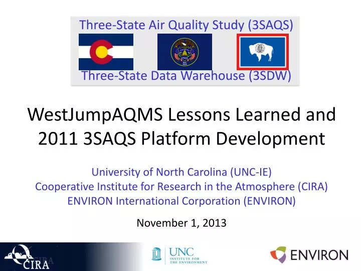
Three-State Air Quality Study (3SAQS) Three-State Data Warehouse (3SDW). WestJumpAQMS Lessons Learned and 2011 3SAQS Platform Development University of North Carolina (UNC-IE) Cooperative Institute for Research in the Atmosphere (CIRA) ENVIRON International Corporation (ENVIRON )

E N D
Three-State Air Quality Study (3SAQS)Three-State Data Warehouse (3SDW) WestJumpAQMS Lessons Learned and 2011 3SAQS Platform Development University of North Carolina (UNC-IE) Cooperative Institute for Research in the Atmosphere (CIRA) ENVIRON International Corporation (ENVIRON) November 1, 2013
Outline • Review the 3SAQS activities for 2011 platform and projections • WestJumpAQMS lessons learned for the 3SAQS modeling protocol • Expectations for the 2013-2014 3SAQS modeling work • Preliminary outline and schedule for 2011 3SAQS modeling
Plans for 2011 platform • Start with development of new protocols for meteorology, emissions, and air quality modeling • Include warehousing and analysis of data in the 3SDW • Projections for emissions • Seeking engagement with stakeholders in this process • Use NEI as the basis of the 3SAQS 2011 emissions data • Include updates for 3SAQS Base 2008 ancillary data • Targeted comparisons between NEI2011 and 3SAQS 2008 inventory in the 3 states: largest sources by county/sector/SCC • Remove/replace key sectors: oil & gas, fires, biogenic
Plans for 2011 platform • 2018 projections off NEI2011 for the 3SAQS 2020 projection modeling • Target changes in the 3 states and compare to changes from the 2008 modeling/projections • 3SAQS 2011 Phase 2 O&G projections for 2020 • Supplemental, targeted surveys for important sources with greatest uncertainties • Include information from existing RMPs • Projections to multiple future years from 2011 • Periodic calls through the process to update and engage 3SAQS stakeholders
Applicable Lessons Learned from WestJumpAQMS • WestJumpAQMS was a very large Photochemical Grid Modeling (PGM) study involving three modeling centers, 100s of Terabytes of data and 100s of stakeholders • The study encountered numerous issues that had to be overcome whose information could benefit other studies • For example, 3SDW/3SAQS, CARMMS. etc. • Chapter 8 of WestJumpAQMS Final Report describes some of the Lessons Learned that is summarized in this presentation
Emissions • Waiting for the NEI2008v2.0 adversely impacted the project • EPA Strongly encouraged WestJumpAQMS to wait for 2008 NEIv2.0 • Not using 2008 NEIv1.5 (May 2011) and waiting for 2008 NEIv2.0 (April 2012) compromised the WestJumpAQMS • Compressed schedule, lost time and resources waiting • Reduction in detail in source apportionment runs • However, in using NEIv2.0 WestJumpAQMS used the most up-to-date emissions available • EPA’s refinement and automation in NEI procedures should make early NEI versions much higher quality than in past
Oil and Gas (O&G) Emissions Inventory (EI) • Outside of WRAP Phase III and Permian Basins relied on NEIv2.0 for O&G emissions • 2008 NEIv2.0 only includes reported (permitted large point) sources and missing lots of O&G emissions • Similar studies to WRAP Phase III O&G EI development should be considered for the rest of the nation • Surveys for WRAP Phase III emissions mainly based on 2006 Baseline conditions • Many changes in O&G development activities since then, such as widespread use of hydraulic fracturing • Incomplete emissions in Phase III O&G EIs • Emissions from evaporation ponds • Fracing and completions • In-field mobile source emissions (P3 Study) • Need for consistent identifiers for sources in tribal and non-tribal areas
On-Road Mobile Sources • Use of SMOKE-MOVES recommended in future as provides day-specific hourly emissions • Coding/script optimizations greatly improves the speed of emissions factor mode processing • Found issues with MOVES inventory-mode monthly emissions due to assumed weekday/weekend day distribution • Use spatial surrogates and temporal profiles that are based on locally collected information
Electrical Generating Unit (EGU) Point Sources • Use hourly Continuous Emissions Monitoring (CEMs) data for large EGU point sources from • CEMs data collected for acid rain trading program to show compliance with the emissions cap • When CEMs malfunctions (missing data), data replaced to maximum emissions • WestJumpAQMS replaced the maximum emissions during missing CEM hours with typical seasonal hourly emissions when the source was operating
Ammonia Emissions • WestJumpAQMS convened an Ammonia Emissions Workgroup to identify improvements (see Memo): • CMU model sufficient • Recommend add bidirectional NH3 flux model to CAMx • Recommend review and update EFs • Recommend collect spatial and activity information on CAFOS and fertilizer applications for model years • Recommend use meteorology in temporal adjustments
Fire Emissions • Final WestJumpAQMS simulations based on the 2008 fire inventory from DEASCO3 study • Preliminary runs used the 2008 Fire Inventory from NCAR (FINN) • Early on WestJumpAQMS compared 2008 FINN with 2008 SMARTFIRE (BlueSky) from the 2008 NEI and found: • FINN was more complete spatially (e.g., Can/Mex) and chemically (see Emissions Technical Memorandum No. 5) • FINN and SMARTFIRE has ~2x the emissions in DEASCO3 • Mainly due to higher emissions for large fires • Exacerbates PM overestimation bias when fire plumes impact PM monitors
Canada Emissions • WestJumpAQMS used 2006 Environment Canada (EC) emissions inventory • No process information (e.g., SCCs) for point sources so had to use default temporal allocation (24/7) • 2008 EC points came speciated for CB05 • According to the 2008 EC emissions file, a Fugitive Dust Transport Factor (FDTF) of 0.25 was applied for dust sources • However, in reality no such FDTF was applied so dust emissions in Canada are overstated by a factor of ~4 • Alberta Environment is working on a 2010 inventory that should be used for future modeling studies: • Should reach out to EC and other Provinces for emission updates • Check high CH4 emissions in central provinces
Mexico Emissions • Last comprehensive emissions inventory for Mexico was for 1999 • WestJumpAQMS used a 2008 Mexico emissions inventory published in 2009 that was projected from the 1999 inventory • It seems like time for a Mexico emissions inventory update • INE has an inventory developed in-house • Marty Wolf at ERG is looking for funding to update the MNEI
Emissions Modeling (SMOKE) • SMOKE emissions modeling was split into numerous streams of emissions by major source category • Easy to identify misplaced emissions • For example, county swapping of O&G emissions in San Juan and Sandoval Counties, NM • Easier to QA/QC • Facilitates tagging for Source Apportionment • Merging numerous “un-merged” emission files can take a long time • Stored on different disks in network • Needs to be taken into account for model run times • With fires and off-shore CMV there are lots of point sources • Will continue to use this approach for 3SAQS
WRF Meteorological Modeling • Very large 4 km IMW Domain • ~339 x ~530 • ~8 processor years per run • Ended up using just a small portions of 4 km WRF domain in PGM modeling • Limited sensitivity tests • Large database management
WRF Meteorological Modeling • 2008 36/12/4 km WRF modeling • ~9 Tb disk storage • All models run on redundant data storage (RAID-5) • Long project schedule necessitated data be archived Silent Corruption of WRF output • Errors corrupted WRF output files • Same file size, valid numbers, just wrong values • All processors worked, CAMx stopped due to unrealistic variables • Screened files with range checks to find bad files and re-ran WRF for offending periods • Recommendation: Make external backups of critical model files ASAP after run completions as data can get corrupted
Model Performance Evaluation • Fundamental differences in Modeled and Measurement definitions for PM species • Need better mapping between the two to account for measurement artifacts • e.g., blank correction • Diagnostic Sensitivity Tests: WestJumpAQMS had limited opportunity due to emissions time crunch • Lots of WRF sensitivity tests • Limited PGM sensitivity tests: • CB05 vs. CB6 chemistry • MOZART vs. GEOS-Chem CONUS BCs • FINN vs. DEASCO3 Fires
Source Apportionment Modeling • Computationally Demanding • Had to make sacrifices due to compressed schedule • Role of Transport in Western U.S. • For ozone international and stratospheric intrusion (i.e., CONUS domain BCs) very important in western U.S. typically half or more of the total ozone on high ozone days • For PM international transport also important (e.g., spring Asian dust events) • Interstate transport for ozone and PM also important using CSAPR-type thresholds analysis • Need to keep 36 km CONUS when doing source apportionment so BCs clearly represent international transport and stratospheric ozone intrusion
Use of MATS with Source Apportionment • Using MATS to bring closure across all Source Group contributions to Design Values introduced an “Unexplained” portion • For ozone we can limit “Unexplained” portion by using modeling results for just the grid cell containing the monitor instead of an array of grid cells • For Annual PM2.5 need to separate and label PM components not covered in Source Apportionment modeling: • Blank Corrections, SOA, SS, PBW • For 24-Hour PM2.5 same as above for annual plus several options: • Average across top 2% days • Weighted quarterly contributions by top 2% days • Other?
Source Apportionment Visualization • Source apportionment generates lots of information • Electronic spreadsheets (Excel) developed that allow users to drill down into SA results • User can tailor results using own labels and scales as desired • How to assure integrity of the data with downloaded Excel files? • Migrate to web-based tools for 3SDW/3SAQS • Data Archiving in 3SDW
Expectations for 2013-2014 • Complete 2011 base and projection modeling early in the year • Bring 3SDW online with 2008 and 2011-based modeling data • Routine distribution and archival/cataloging of NEPA and regional modeling studies • Cumulative impacts modeling and analysis • Winter ozone case study • Convene 3SAQS working groups and use feedback to improve modeling process and products
Preliminary Outline • Modeling protocol development – met, emissions, and air quality modeling • Extends and builds on 2008 modeling protocol • Data, modeling process, and evaluation protocol • WRF 2011 modeling and MPE at 36/12/4-km • SMOKE 2011 modeling at 36/12/4-km • Requires NEI2011 and 2011 O&G inventories from Phase I work • SMOKE future year (2020 target year?) modeling at 36/12/4-km • Requires analysis of EPA projections off of 2008 and 2011 and applicability to 3SAQS • Completion of Phase II O&G inventories • Emissions projection curves for each future year from 2018 2025 (correct end year?) • CAMx2011 and future year modeling at 36/12-km • Requires decision on BCs (GEOS-Chem or MOZART) • Base year runs, source apportionment, cumulative impacts, other? • Upload results into 3SDW and distribute to stakeholders