Download
1 / 31
310 likes | 312 Views
This case study explores the use of synthetic jets for flow control in aerodynamics. It includes 2D simulations, grid and modeling issues, and results. The study also mentions future work for 3D simulations.

E N D
CASE 1: TWO-DIMENSIONAL RANS SIMULATION OF A SYNTHETIC JET FLOW FIELD J. Cui and R. K. Agarwal Mechanical & Aerospace Engineering Department Washington University, St. Louis, MO 63130
Outline • Introduction • Software Employed • 2D Simulations of a Synthetic Jet Flow Field • Grid and Modeling Issues • Results and Discussion • Conclusions of 2D Simulation Results • Preliminary 3D Simulations of a Synthetic Jet Flow Field • Future Work
Motivation for Active Flow Control • In recent years, it has been surmised that the fluidic modification of aerodynamic and propulsive flow fields can cover multiple flight regimes without the need of conventional control surfaces such as flaps, spoilers and variable wing sweep. • The fluidic modification (or flow control) can be accomplished by employing micro-surface effectors and other fluidic devices dynamically operated by an intelligent control system. • These new “flow control” technologies thus have the potential of resulting in radical improvement in aircraft performance and weight reduction.
Flow Control with Synthetic Jets • Virtual Aerodynamic Shape Modification of an Airfoil Using a Synthetic Jet Actuator (AIAA 03-4158) • Vectoring Control of a Primary Jet with Synthetic Jets (AIAA 02-3284) • Control of Recirculating Flow Region Behind a Backward Facing Step Using Synthetic Jets (AIAA 03-1125) • Interaction of a Synthetic Jet with a Flat Plate Turbulent Boundary Layer (AIAA 03-3458) • Flow Control of Shear Layers Over 2-D Cavities Using Pulsed Jet (AIAA 04-428)
CFD Flow-Solver Employed • WIND • structured, multi-zone, compressible RANS solver • 2nd or higher-order upwind/central differencing • Four-stage Runge-Kutta time stepping • Spalart-Allmaras (SA), Mentor’s SST, combined SST & LES, and k-ε turbulence models
Grid Employed Zone 4 (197139) Zone 3 (4165) Zone 1 (3386) Zone 2 (6250) Diaphragm Whole view Zoomed in: the grid of the slot
Boundary Conditions • External Flow Region (zone 4) • Bottom wall (except SJ) no-slip • All other threeboundaries outflow • SJ Actuator(zone 1, 2 & 3) • At the diaphragm arbitrary inflow • All other boundaries coupled or no-slip wall • At the Diaphragm (zone 1, I=1)
Justification of Boundary Conditions Mass-flux at the diaphragm & SJ slot Pressure inside the cavity
Justification of Boundary Conditions(cont.) Phase-averaged v-velocity at (x, y) = (0, 0.1 mm)
Time-step & Grid Independence Studies Long-time averaged v-velocity along the centerline Phase-averaged v-velocity at (0, 2mm)
Long-time Averagedv-Velocity along the Centerline (a) v-velocity along the centerline (b) Zoomed-in view: near the wall
Long-time Averagedv-Velocity along x-Axis y = 0.1mm y = 1mm
Averaged Jet Width & Phase-Averagedv-Velocity Averaged jet width Phase-averagedv-velocity
Phase-Averaged Velocity Contours(uat 45) PIV data SST SST_LES SA
Phase-Averaged Velocity Contours(vat 45) PIV data SST SST_LES SA
Phase-Averaged Velocity Contours(uat 90) PIV data SST SST_LES SA
Phase-Averaged Velocity Contours(vat 90) PIV data SST SST_LES SA
Phase-Averaged Velocity Contours(vat 135) PIV data SST SST_LES SA
Phase-Averaged Velocity Contours(vat 225) PIV data SST SST_LES SA
Conclusions of 2D Simulation Results • 2D RANS simulations (SST, SST_LES, SA) and experiments have reasonable agreement in capturing the overall features of the flow field. • SST model gives the best result out of three simulations
Preliminary 3D Simulations • Grids • Modeling issues (same as in 2D simulations) • Results and discussions
Grid Employed y z x Zone 3 (296135) 5 7 9 Zone 1 (731117) 4 6 8 y Diaphragm Zone 2 (191951) x Whole view (9 zones) Zoomed in: the grid of the slot
Long-time Averagedv-Velocity along x-Axis y = 1mm y = 0.1mm
Averaged Jet Width & Phase-Averagedv-Velocity Averaged jet width Phase-averagedv-velocity
Phase-Averaged Velocity Contours (u, vat 45) PIV data 2D SST 3D SST u v
Phase-Averaged Velocity Contours (u, vat 90) PIV data 2D SST 3D SST u v
Phase-Averaged Velocity Contours (vat 135, 225) PIV data 2D SST 3D SST 135 225
Future Work • 3D simulations of case1: time-step and grid refinement study • 3D simulations of case 2: synthetic jet interacts with cross flow