Download
1 / 60
1.13k likes | 1.63k Views
ELECTROCHEMICAL IMPEDANCE SPECTROSCOPY. Introduction.

E N D
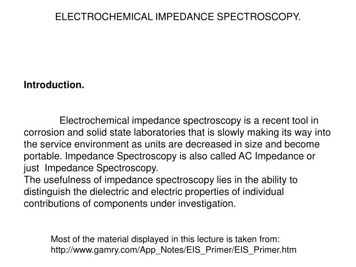
ELECTROCHEMICAL IMPEDANCE SPECTROSCOPY. Introduction. Electrochemical impedance spectroscopy is a recent tool in corrosion and solid state laboratories that is slowly making its way into the service environment as units are decreased in size and become portable. Impedance Spectroscopy is also called AC Impedance or just Impedance Spectroscopy. The usefulness of impedance spectroscopy lies in the ability to distinguish the dielectric and electric properties of individual contributions of components under investigation. Most of the material displayed in this lecture is taken from: http://www.gamry.com/App_Notes/EIS_Primer/EIS_Primer.htm
ELECTROCHEMICAL IMPEDANCE SPECTROSCOPY For example, if the behavior of a coating on a metal when in salt water is required, by the appropriate use of impedance spectroscopy, a value of resistance and capacitance for the coating can be determined through modeling of the electrochemical data. The modeling procedure uses electrical circuits built from components such as resistors and capacitors to represent the electrochemical behavior of the coating and the metal substrate. Changes in the values for the individual components indicate their behavior and performance. Impedance spectroscopy is a non-destructive technique and so can provide time dependent information about the properties but also about ongoing processes such as corrosion or the discharge of batteries and e.g. the electrochemical reactions in fuel cells, batteries or any other electrochemical process.
ELECTROCHEMICAL IMPEDANCE SPECTROSCOPY. Below is a listing of the advantages and disadvantages of the technique. Advantages. 1. Useful on high resistance materials such as paints and coatings. 2. Time dependent data is available 3. Non- destructive. • Quantitative data available. • Use service environments. Disadvantages. 1. Expensive. 2. Complex data analysis for quantification.
Five major topics are covered in this application note • AC Circuit Theory and Representation of Complex Impedance Values. • Physical Electrochemistry and Circuit Elements. • Common Equivalent Circuit Models. • Extracting Model Parameters from Impedance Data. • Case studies
AC Circuit Theory and Representation of Complex Impedance Values Impedance definition: concept of complex impedance Ohm's law defines resistance in terms of the ratio between voltage E and current I. The relationship is limited to only one circuit element -- the ideal resistor. An ideal resistor has several simplifying properties: • It follows Ohm's Law at all current and voltage levels • It's resistance value is independent of frequency. • AC current and voltage signals though a resistor are in phase with each other
Real World: • Circuit elements that exhibit much more complex behavior. These elements force us to abandon the simple concept of resistance. In its place we use impedance, which is a more general circuit parameter. • Like resistance, impedance is a measure of the ability of a circuit to resist the flow of electrical current. Unlike resistance, impedance is not limited by the simplifying properties listed above. • Electrochemical impedance is usually measured by applying an AC potential to an electrochemical cell and measuring the current through the cell. • Suppose that we apply a sinusoidal potential excitation. The response to this potential is an AC current signal, containing the excitation frequency and it's harmonics. This current signal can be analyzed as a sum of sinusoidal functions (a Fourier series). • Electrochemical Impedance is normally measured using a small excitation signal. This is done so that the cell's response is pseudo-linear. Linearity is described in more detail in a following section. In a linear (or pseudo-linear) system, the current response to a sinusoidal potential will be a sinusoid at the same frequency but shifted in phase.
Sinusoidal Current Response in a Linear System The excitation signal, expressed as a function of time, has the form of: E(t) is the potential at time tr Eo is the amplitude of the signal, and is the radial frequency. The relationship between radial frequency (expressed in radians/second) and frequency f (expressed in Hertz (1/sec).
Impedance as a Complex Number Z(,Vo) = V() / I() • The impedance at any frequency is a complex number because I() contains phase information as well as magnitude - the AC current may have a phase lag with respect to the AC voltage If we apply V=Vo + V xcos( t) and measure I = Io + I cos( t- ) Then: Z(,Vo) = (V / I ) x{cos() + i sin()} where i2 = -1 and both magnitude and phase of the impedance, Z and vary with
Response in a linear System In a linear system, the response signal, the current I(t), is shifted in phase () and has a different amplitude, I0: An expression analogous to Ohm's Law allows us to calculate the admittance (=the AC resistance) of the system : The impedance is therefore expressed in terms of a magnitude, Z0, and a phase shift, f. This admittance may allso be written as complex function:
Measure Z(,Vbias) The result will be Z(,Vo) = V() / I()
Response dI of dE from the Current (I)/Field (E) relation: Let us assume we have an electrical element to which we apply an electric field E(t) and get the response I(t), then we can disturb this system at a certain field E with a small perturbation dE and we will get at the current I a small response perturbation dI. In the first approximation, as the perturbation dE is small, the response dI will be a linear response as well (mirror at the tangent oft the I(E) curve! If we plot the applied sinusoidal signal on the X-axis of a graph and the sinusoidal response signal I(t) on the Y-axis, an oval is plotted. This oval is known as a "Lissajous figure". Analysis of Lissajous figures on oscilloscope screens was the accepted method of impedance measurement prior to the availability of lock-in amplifiers and frequency response analyzers.
Complex writing Using Eulers relationship it is possible to express the impedance as a complex function. The potential is described as, and the current response as, The impedance is then represented as a complex number,
Data Presentation:Nyquist Plot with Impedance Vector Look at the Equation above. The expression for Z() is composed of a real and an imaginary part. If the real part is plotted on the X axis and the imaginary part on the Y axis of a chart, we get a "Nyquist plot". Notice that in this plot the y-axis is negative and that each point on the Nyquist plot is the impedance Z at one frequency. On the Nyquist plot the impedance can be represented as a vector of length |Z|. The angle between this vector and the x-axis is f. Nyquist plots have one major shortcoming. When you look at any data point on the plot, you cannot tell what frequency was used to record that point. Low frequency data are on the right side of the plot and higher frequencies are on the left. This is true for EIS data where impedance usually falls as frequency rises (this is not true of all circuits). The Nyquist plot the results from the RC circuit. The semicircle is characteristic of a single "time constant". Electrochemical Impedance plots often contain several time constants. Often only a portion of one or more of their semicircles is seen.
The Bode Plot Another popular presentation method is the "Bode plot". The impedance is plotted with log frequency on the x-axis and both the absolute value of the impedance (|Z| =Z0 ) and phase-shift on the y-axis. The Bode plot for the RC circuit is shown below. Unlike the Nyquist plot, the Bode plot explicitly shows frequency information.
The different views on impedance data The impedance data are the red points. Their projection onto the Z“-Z‘ plane is called the Nyquist plot The projection onto the Z“- plane is called the Cole Cole diagram Z” Nyquist plot Cole Cole diagram Z´ Bode plot
Electrochemistry - A Linear System? • Electrical circuit theory distinguishes between linear and non-linear systems (circuits). Impedance analysis of linear circuits is much easier than analysis of non-linear ones. • A linear system ... is one that possesses the important property of superposition: If the input consists of the weighted sum of several signals, then the output is simply the superposition, that is, the weighted sum, of the responses of the system to each of the signals. • Mathematically, let y1(t) be the response of a continuous time system to x1(t) ant let y2(t) be the output corresponding to the input x2(t). • Then the system is linear if: • The response to x1(t) + x2(t) is y1(t) + y2(t) • 2) The response to ax1(t) is ay1(t) ...
Current versus Voltage Curve Showing Pseudo-linearity For a potentiostated electrochemical cell, the input is the potential and the output is the current. Electrochemical cells are not linear! Doubling the voltage will not necessarily double the current. However, we will show how electrochemical systems can be pseudo-linear. When you look at a small enough portion of a cell's current versus voltage curve, it seems to be linear. In normal EIS practice, a small (1 to 10 mV) AC signal is applied to the cell. The signal is small enough to confine you to a pseudo-linear segment of the cell's current versus voltage curve. You do not measure the cell's nonlinear response to the DC potential because in EIS you only measure the cell current at the excitation frequency.
Steady State Systems Measuring an EIS spectrum takes time (often many hours). The system being measured must be at a steady state throughout the time required to measure the EIS spectrum. A common cause of problems in EIS measurements and their analysis is drift in the system being measured. In practice a steady state can be difficult to achieve. The cell can change through adsorption of solution impurities, growth of an oxide layer, build up of reaction products in solution, coating degradation, temperature changes, to list just a few factors. Standard EIS analysis tools may give you wildly inaccurate results on a system that is not at a steady state
Time and Frequency Domains and Transforms Signal processing theory refers to data domains. The same data can be represented in different domains. In EIS, we use two of these domains, the time domain and the frequency domain. In the time domain, signals are represented as signal amplitude versus time. The Figure demonstrates this for a signal consisting of two superimposed sine waves. Two Sine Waves in the Time Domain
Time and frequency domain The figures show the same data of the two sinus waves in the time and the frequency domain. Two Sine Waves in the Time Domain Amplitude Time Two Sine Waves in the Frequency Domain Amplitude Frequency Use the Fourier transform and inverse Fourier transform to switch between the domains. The common term, FFT, refers to a fast, computerized implementation of the Fourier transform. Detailed discussion of these transforms is beyond the scope of this manual. Several of the references given at the end of this chapter contain more information on the Fourier transform and its use in EIS. In modern EIS systems, lower frequency data are usually measured in the time domain. The controlling computer applies a digital approximation to a sine wave to the cell by means of a digital to analog converter. The current response is measured using an analog to digital computer. An FFT is used to convert the current signal into the frequency domain.
Electrical Circuit Elements EIS data is commonly analyzed by fitting it to an equivalent electrical circuit model. Most of the circuit elements in the model are common electrical elements such as resistors, capacitors, and inductors. To be useful, the elements in the model should have a basis in the physical electrochemistry of the system. As an example, most models contain a resistor that models the cell's solution resistance. Some knowledge of the impedance of the standard circuit components is therefore quite useful. The Table lists the common circuit elements, the equation for their current versus voltage relationship, and their impedance: Notice that the impedance of a resistor is independent of frequency and has only a real component. Because there is no imaginary impedance, the current through a resistor is always in phase with the voltage. The impedance of an inductor increases as frequency increases. Inductors have only an imaginary impedance component. As a result, an inductor's current is phase shifted 90 degrees with respect to the voltage. The impedance versus frequency behavior of a capacitor is opposite to that of an inductor. A capacitor's impedance decreases as the frequency is raised. Capacitors also have only an imaginary impedance component. The current through a capacitor is phase shifted -90 degrees with respect to the voltage.
Serial and Parallel Combinations of Circuit Elements Very few electrochemical cells can be modeled using a single equivalent circuit element. Instead, EIS models usually consist of a number of elements in a network. Both serial and parallel combinations of elements occur. Impedances in Series: Impedances in Parallel
Serial and Parallel Combinations of Circuit Elements Suppose we have a 1 and a 4 resistor is series. The impedance of a resistor is the same as its resistance (see Table 2-1). We thus calculate the total impedance Zeq: R1 R2 Resistance and impedance both go up when resistors are combined in series. Now suppose that we connect two 2 µF capacitors in series. The total capacitance of the combined capacitors is 1 µF C1 C2 Impedance goes up, but capacitance goes down when capacitors are connected in series. This is a consequence of the inverse relationship between capacitance and impedance.
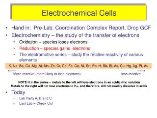
Example: The Zn Air battery There are three reactions: • The reaction at the anode between metal ions and electrons : • The reaction at the cathode between water and electrons • The reaction of the whole cell, i.e. the two half-cell reactions added together:
An electrochemical cell: The Zn Air battery For each of these reactions it is true that: where:G is the free energy change of the reaction.G0 is what the free energy change would be if every component were in its standard state. ax is the activity of reaction product X and ay is the activity of reactant Y. nx is the stoichiometric coefficient of reaction product X, and likewise for the reactants.(The stoichiometric coefficient is the number of that molecule that are involved in the reaction; for the whole-cell reaction written above, the stoichiometric coefficient of water is 2, and of oxygen gas is 1.)R is the ideal gas constant and T is the temperature.The symbol is the multiplying equivalent of : all the terms after it are multiplied together.
An electrochemical cell: The Zn Air battery Equilibrium If a reaction is at equilibrium, G=0 , and the free energy G of the system is at a minimum with respect to how much of the reactants have been converted to products. When this is the case, we obtain: where K is the equilibrium constant. Thus we can deduce that G0 =RTlnk ; this is true of a reaction whether it is at equilibrium or not. (G0 for a reaction is determined by the energies of the bonds within the molecules of the reactants and products, and this is independent of how many such molecules there are per unit volume.)
The Zn Air battery: An electrochemical cell The cathode reaction is at equilibrium if there is no power supply connected to the circuit. It can do this because each atom or ion has enough energy to undergo the reaction in either direction; there is nothing stopping it being at equilibrium. The anode reaction is also at its own equilibrium. The reaction for the whole cell is not at equilibrium. There is too much of an energy barrier for it to be able to get there – the ions have to diffuse through the electrolyte and the electrons have to go around through the wires. (Or through a high impedance voltmeter, which they almost certainly cannot do.) Thus for the example given: G 0 and the quotient is not the equilibrium constant but equal to the electric potential. We can convert this into an expression for the electrical potentials using the general rule: where z is the stoichiometric number of electrons in the reaction. (This is due to Faraday’s law)
An electrochemical cell: The Zn Air battery In this form we have the Nernst equation for the cell and : The activities of Zn and water are one, because Zn is in its standard state and the water is so much more abundant than its solutes that it may as well be in its standard state. Thus: E0 is the equilibrium potential – it is the potential of the whole cell when the electrodes are at equilibrium within themselves. It can be worked out (easily, using algebra with a pen and pencil) that: where K is the equilibrium constant – i.e. if we were at equilibrium over the whole electrochemical cell, then E would be zero. E0 is a property of the system like that G0 , and is still equal to the same number even when the whole cell is not at equilibrium. If for some reason it was required to find the value of E0 , we could use this expression. E0 is called the standard electrode potential.
Physical Electrochemistry and Equivalent Circuit Elements Electrolyte Resistance: Electrolyte resistance is often a significant factor in the impedance of an electrochemical cell. A modern 3 electrode potentiostat compensates for the solution resistance between the counter and reference electrodes. However, any solution resistance between the reference electrode and the working electrode must be considered when you model your cell. The resistance of an ionic solution depends on the ionic concentration, type of ions, temperature and the geometry of the area in which current is carried. In a bounded area with area A and length l carrying a uniform current the resistance is defined as:
The electrolyte resisatnce Standard chemical handbooks list values for specific solutions. For other solutions and solid materials, you can calculate from specific ion conductances. The units for are Siemens per meter (S/m). The Siemens is the reciprocal of the ohm, so 1 S = 1/ohm Unfortunately, most electrochemical cells do not have uniform current distribution through a definite electrolyte area. The major problem in calculating solution resistance therefore concerns determination of the current flow path and the geometry of the electrolyte that carries the current. A comprehensive discussion of the approaches used to calculate practical resistances from ionic conductances is well beyond the scope of this manual. Fortunately, you don't usually calculate solution resistance from ionic conductances. Instead, it is found when you fit a model to experimental EIS data.
Double Layer Capacitance A electrical double layer exists at the interface between an electrode and its surrounding electrolyte. This double layer is formed as ions from the solution "stick on" the electrode surface. Charges in the electrode are separated from the charges of these ions. The separation is very small, on the order of angstroms. Charges separated by an insulator form a capacitor. On a bare metal immersed in an electrolyte, you can estimate that there will be approximately 30 µF of capacitance for every cm2 of electrode area. The value of the double layer capacitance depends on many variables including electrode potential, temperature, ionic concentrations, types of ions, oxide layers, electrode roughness, impurity adsorption, etc. Principle of the Electric Double-Layer: Here C electrodes
Polarization Resistance Whenever the potential of an electrode is forced away from it's value at open circuit, that is referred to as polarizing the electrode. When an electrode is polarized, it can cause current to flow via electrochemical reactions that occur at the electrode surface. The amount of current is controlled by the kinetics of the reactions and the diffusion of reactants both towards and away from the electrode. In cells where an electrode undergoes uniform corrosion at open circuit, the open circuit potential is controlled by the equilibrium between two different electrochemical reactions. One of the reactions generates cathodic current and the other anodic current. The open circuit potential ends up at the potential where the cathodic and anodic currents are equal. It is referred to as a mixed potential. The value of the current for either of the reactions is known as the corrosion current.
The Butler Volmer equation: For the polarization resistance of simple reactions at electrodes When there are two simple, kinetically controlled reactions occurring, the potential of the cell is related to the current by the following (known as the Butler-Volmer equation). I is the measured cell current in amps,Icorr is the corrosion current in amps,Eoc is the open circuit potential in volts,a is the anodic Beta coefficient in volts/decade,c is the cathodic Beta coefficient in volts/decade If we apply a small signal approximation (E-Eoc is small) to the buler Volmer equation, we get the following: which introduces a new parameter, Rp, the polarization resistance. As you might guess from its name, the polarization resistance behaves like a resistor. If the Tafel constants i are known, you can calculate the Icorr from Rp. The Icorr in turn can be used to calculate a corrosion rate. We will further discuss the Rp parameter when we discuss cell models.
Charge Transfer Resistance A similar resistance is formed by a single kinetically controlled electrochemical reaction. In this case we do not have a mixed potential, but rather a single reaction at equilibrium. Consider a metal substrate in contact with an electrolyte. The metal molecules can electrolytically dissolve into the electrolyte, according to: or more generally: In the forward reaction in the first equation, electrons enter the metal and metal ions diffuse into the electrolyte. Charge is being transferred. This charge transfer reaction has a certain speed. The speed depends on the kind of reaction, the temperature, the concentration of the reaction products and the potential. The general relation between the potential and the current holds: io = exchange current density Co = concentration of oxidant at the electrode surface Co* = concentration of oxidant in the bulk CR = concentration of reductant at the electrode surface F = Faradays constant T = temperature R = gas constant a = reaction order n = number of electrons involvedh = overpotential ( E - E0 )
Overvoltage potential The overpotential, h, measures the degree of polarization. It is the electrode potential minus the equilibrium potential for the reaction. When the concentration in the bulk is the same as at the electrode surface, Co=Co* and CR=CR*. This simplifies the last equation into: This equation is called the Butler-Volmer equation. It is applicable when the polarization depends only on the charge transfer kinetics. Stirring will minimize diffusion effects and keep the assumptions of Co=Co* and CR=CR* valid. When the overpotential, h, is very small and the electrochemical system is at equilibrium, the expression for the charge transfer resistance changes into: From this equation the exchange current i0 density can be calculated when Rct is known.
Diffusion: Warburg impedance with infinite thickness Diffusion can create an impedance known as the Warburg impedance. This impedance depends on the frequency of the potential perturbation. At high frequencies the Warburg impedance is small since diffusing reactants don't have to move very far. At low frequencies the reactants have to diffuse farther, thereby increasing the Warburg impedance. The equation for the "infinite" Warburg impedance On a Nyquist plot the infinite Warburg impedance appears as a diagonal line with a slope of 0.5. On a Bode plot, the Warburg impedance exhibits a phase shift of 45°. In the above equation, s is the Warburg coefficient defined as: = radial frequency DO = diffusion coefficient of the oxidant DR = diffusion coefficient of the reductant A = surface area of the electrode n = number of electrons transferred C* = bulk concentration of the diffusing species (moles/cm3)
Coating Capacitance A capacitor is formed when two conducting plates are separated by a non-conducting media, called the dielectric. The value of the capacitance depends on the size of the plates, the distance between the plates and the properties of the dielectric. The relationship is: With, o = electrical permittivity r = relative electrical permittivity A = surface of one plate d = distances between two plates Whereas the electrical permittivity is a physical constant, the relative electrical permittivity depends on the material. Some useful r values are given in the table: Notice the large difference between the electrical permittivity of water and that of an organic coating. The capacitance of a coated substrate changes as it absorbs water. EIS can be used to measure that change
Constant Phase Element (for double layer capacity in real electrochemical cells) Capacitors in EIS experiments often do not behave ideally. Instead, they act like a constant phase element (CPE) as defined below. When this equation describes a capacitor, the constant A = 1/C (the inverse of the capacitance) and the exponent = 1. For a constant phase element, the exponent a is less than one. The "double layer capacitor" on real cells often behaves like a CPE instead of like a capacitor. Several theories have been proposed to account for the non-ideal behavior of the double layer but none has been universally accepted. In most cases, you can safely treat as an empirical constant and not worry about its physical basis.
Common Equivalent Circuit Models In the following section we show some common equivalent circuits models. To elements used in the following equivalent circuits are presented in the Table. Equations for both the admittance and impedance are given for each element.
A Purely Capacitive Coating A metal covered with an undamaged coating generally has a very high impedance. The equivalent circuit for such a situation is in the Figure: C R The model includes a resistor (due primarily to the electrolyte) and the coating capacitance in series. A Nyquist plot for this model is shown in the Figure. In making this plot, the following values were assigned: R = 500 (a bit high but realistic for a poorly conductive solution)C = 200 pF (realistic for a 1 cm2 sample, a 25 µm coating, and r = 6 )fi = 0.1 Hz (lowest scan frequency -- a bit higher than typical) ff = 100 kHz (highest scan frequency) The value of the capacitance cannot be determined from the Nyquist plot. It can be determined by a curve fit or from an examination of the data points. Notice that the intercept of the curve with the real axis gives an estimate of the solution resistance. The highest impedance on this graph is close to 1010. This is close to the limit of measurement of most EIS systems
A Purely Capacitive Coating in the Bode Plot The same data are shown in a Bode plot in Figure 2-13. Notice that the capacitance can be estimated from the graph but the solution resistance value does not appear on the chart. Even at 100 kHz, the impedance of the coating is higher than the solution resistance
The Voigt network An electrical layer of a device can often be described by a resistor and capacitor in parallel
Cole-Cole Plots: Impedance Plots in the Complex Plane When we plot the real and imaginary components of impedance in the complex plane (Argand diagram), we obtain a semicircle or partial semicircle for each parallel RC Voigt network: The diameter corresponds to the resistance R. The frequency at the 90° position corresponds to 1/t = 1/RC
Analyzing Circuits By using the various Cole-Cole plots we can calculate values of the elements of the equivalent circuit for any applied bias voltage By doing this over a range of bias voltages, we can obtain: the field distribution in the layers of the device (potential divider) and the relative widths of the layers, since C ~ 1/d
Randles Cell The Randles cell is one of the simplest and most common cell models. It includes a solution resistance, a double layer capacitor and a charge transfer or polarization resistance. In addition to being a useful model in its own right, the Randles cell model is often the starting point for other more complex models. The equivalent circuit for the Randles cell is shown in the Figure. The double layer capacity is in parallel with the impedance due to the charge transfer reaction The Nyquist plot for a Randles cell is always a semicircle. The solution resistance can found by reading the real axis value at the high frequency intercept. This is the intercept near the origin of the plot. Remember this plot was generated assuming that Rs = 20 and Rp= 250 . The real axis value at the other (low frequency) intercept is the sum of the polarization resistance and the solution resistance. The diameter of the semicircle is therefore equal to the polarization resistance (in this case 250 ).
Bode Plot oft Randalls cell This Figure is the Bode plot for the same cell. The solution resistance and the sum of the solution resistance and the polarization resistance can be read from the magnitude plot. The phase angle does not reach 90° as it would for a pure capacitive impedance. If the values for Rs and Rp were more widely separated the phase would approach 90°. Bode Plot for 1 mm/year Corrosion Rate
Mixed Kinetic and Diffusion Control First consider a cell where semi-infinite diffusion is the rate determining step, with a series solution resistance as the only other cell impedance. A Nyquist plot for this cell is shown in Figure 2-17. Rs was assumed to be 20 W. The Warburg coefficient calculated to be about 120 sec-1/2 at room temperature for a two electron transfer, diffusion of a single species with a bulk concentration of 100 µM and a typical diffusion coefficient of 1.6 x10⁻⁵ cm2/sec. Notice that the Warburg Impedance appears as a straight line with a slope of 45°.
Example: Half a fuel cell Adding to the previous example a double layer with capacitance and a charge transfer impedance, we get the equivalent circuit: This circuit models a cell where polarization is due to a combination of kinetic and diffusion processes. The Nyquist plot for this circuit is shown in the Figure. As in the above example, the Warbug coefficient is assumed to be about 150 W sec-1/2. Other assumptions: Rs = 20 , Rct = 250 , and Cdl = 40 µF.
Bode plot The Bode plot for the same data is shown here. The lower frequency limit was moved down to 1mHz to better illustrate the differences in the slope of the magnitude and in the phase between the capacitor and the Warburg impedance. Note that the phase approaches 45° at low frequency.
Case studies • Relaxation Dispersion of O2- Ionic Conductivity in a ZrO0.85Ca0.15O1.85 Single Crystal • Effect of intergranular glass films on the electrical conductivityof 3Y-TZP