Taxonomic

1. Modern Comparative Methods Taxonomic Phylogenetic

2. Modern Comparative Methods Taxonomic Phylogenetic Analysis of Covariance Nested ANOVA

3. [Source: Garland 2001, pp. 107-132 in Hypoxia: From Genes to the Bedside, Academic Press, NY]

4. Modern Comparative Methods Taxonomic Phylogenetic Analysis of Covariance Nested ANOVA

5. [Source: Dunham & Miles 1985, Am Nat. 126: 231-257]

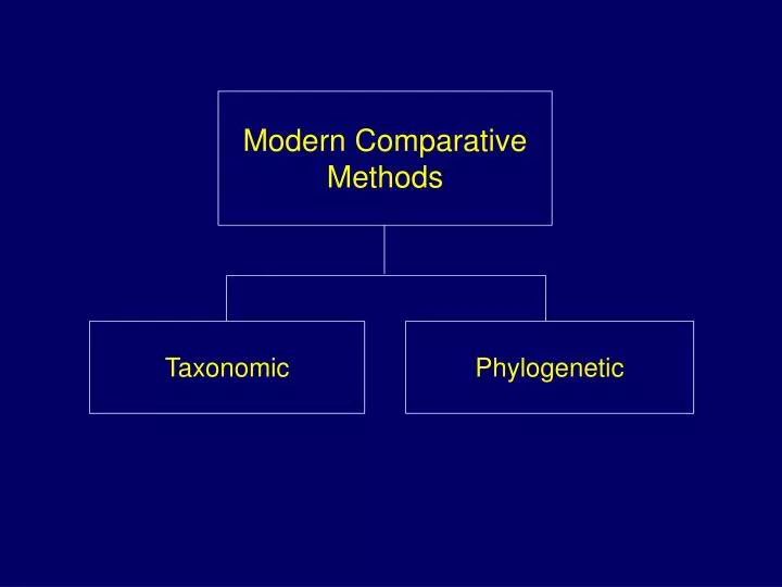
6. Modern Comparative Methods Taxonomic Phylogenetic Generalized Linear Models Independent Contrasts

7. Cheverud et al. (1985) Grafen (1989) General Linear Model y = a + βx1 + βx2…βxn + ε Mean structure Error structure [Source: Martins & Hansen 1997, Am. Nat. 149: 646-667]

8. not additive Components of Error • Error in measurement of X’s and Y • Error due to stochastic evolutionary processes • Error due to imperfect phylogenetic information (topology or branch lengths) additive [Source: Martins & Hansen 1997, Am. Nat. 149: 646-667]

9. Modern Comparative Methods Taxonomic Phylogenetic Generalized Linear Models Independent Contrasts

10. Independent Contrasts • A set of N-1 phylogenetically independent data points • Can be used in any univariate or multivariate analyses • Yield identical statistical power as do analyses of raw data [Source: Felsenstein 1985, Amer. Nat. 125: 1-15]

11. XA XB XC XD A B C D Independent contrasts for trait Xi, where i is the specific taxon. The value of XA and XB are not independent But XA-XB is clearly independent of XC-XD. These two values are independent contrasts. [Source: Felsenstein 1985, Amer. Nat. 125: 1-15]

12. XA XB XC XD A B C D XE = (1/vA)XA + (1/vB)XB 1/vA + 1/vB Independent contrasts for trait Xi, where i is the specific taxon. The value of Xi for an ancestor (e.g., E) is the weighted mean of Xi for the descendants. vA vB E F [Source: Felsenstein 1985, Amer. Nat. 125: 1-15]

13. What do you need to compute independent contrasts? • A fully resolved cladogram • Branch lengths • Data for two or more traits [Source: Garland et al. 1992, Syst. Biol. 41: 18-32]

14. Standardizing Contrasts • Taxa that have been separated by longer periods of time should have larger contrasts. • Must standardize contrasts before using them in statistical analyses (mean = 0, variance = 1). • Because the expected mean of contrasts is zero, all you need to do is divide the contrasts by their standard deviation (= square root of the sum of branch lengths) [Source: Garland et al. 1992, Syst. Biol. 41: 18-32]

15. Assessing Standardization Adequate standardization is assessed by regressing standardized contrasts onto the standard deviation of a contrast (square root of the sum of branch lengths) A correlation (+ or -) implies inadequate standardization. [Source: Garland et al. 1992, Syst. Biol. 41: 18-32]

16. Use of Contrasts in Statistical Analyses • Contrasts can be used in any subsequent statistical analyses as you would use raw data. • However, the following restrictions hold: • All standard assumptions of parametric statistics (e.g., homoscedasticity, normality of residuals) also apply to the analysis of contrasts. • Statistical models should not include an intercept because the intercept of a relationship between two sets of contrasts is theoretically equal to zero. [Source: Garland et al. 1992, Syst. Biol. 41: 18-32]

17. Can contrasts be computed for environmental variables? • Some have argued that the use of contrasts for environmental variables is inappropriate (e.g., see Martins 2000). • Garland et al. (1992) noted that contrasts could be computed for a continuous environmental variable if environmental states are passed from ancestor to descendant. [Sources: Martins 2000, Trends Ecol. Evol. 15: 296-299; Garland et al. 1992, Syst. Biol. 41: 18-32]

18. [Source: Angilletta et al. 2004, Am. Nat. 164: in press]

19. Can contrasts be used for intraspecific comparisons? • When gene flow among populations is limited, phylogenetic comparative methods can be applied in studies of microevolution. • Alternatively, Felsenstein (2002) proposed a method of computing contrasts for intraspecific data that accounts for gene flow among populations. [Source: Niewiarowski et al. 2004, Evolution 58: 619-633]

20. VT = VP + VS + 2[cov(P,S)] Phylogenetic Autocorrelation VT = total variance VP = phylogenetic variance VS = specific variance cov(P,S) = covariance between phylogenetic and specific values [Source: Cheverud et al. 1985, Evolution 39: 1335-1351] [Source: Cheverud et al. 1985, Evolution 39: 1335-1351]

21. y = pWy + e Phylogenetic similarity Phylogenetic Autocorrelation y = vector of standardized trait values (n x 1) p = phylogenetic autocorrelation coefficient W = matrix of phylogenetic connectivity (n x n) e = vector of residual trait values [Source: Cheverud et al. 1985, Evolution 39: 1335-1351] [Source: Cheverud et al. 1985, Evolution 39: 1335-1351]

22. Interpreting the Autocorrelation Coefficient P The autocorrelation coefficient is standardized like a typical correlation coefficient: -1 ≤ p≤ 1 p = 0 → no phylogenetic effect 0<p ≤ 1 → phylogenetic similarity -1 ≤p < 0 → phylogenetic dissimilarity [Source: Cheverud et al. 1985, Evolution 39: 1335-1351]

23. Examples of Autocorrelation Coefficients [Source: Cheverud et al. 1985, Evolution 39: 1335-1351]

24. Do different methods yield similar results? [Source: Niewiarowski et al. 2004, Evolution 58: 619-633]

25. Do different methods yield similar results? [Source: Niewiarowski et al. 2004, Evolution 58: 619-633]

26. Are phylogenetic methods necessary? • Some biologists have argued that phylogenetic comparative methods are too conservative • If the phylogenetic information is imperfect, a comparative method could be misleading. • One recommendation is to investigate the extent of phylogenetic signal prior to choosing a comparative method.

27. Phylogenetic Signal (K) If a trait evolves according to a model of Brownian motion, then K = 1. [Source: Blomberg et al. 2003, Evolution 57: 717-745]

28. [Source: Garland 2001, pp. 107-132 in Hypoxia: From Genes to the Bedside, Academic Press, NY] [See also Garland et al. 1999, Am. Zool. 39: 374-388]