Download

1 / 14
140 likes | 245 Views
Paul Vitanyi CWI, University of Amsterdam. Similarity and Denoising. Problem 1: Similarity. Given : Literal objects. ( binary files ). 2. 1. 3. 4. 5. :. Determine : “Similarity” Distance Matrix (distances between every pair).

E N D
Paul VitanyiCWI, University of Amsterdam Similarity and Denoising
Problem 1: Similarity Given: Literal objects (binary files) 2 1 3 4 5 : Determine: “Similarity” Distance Matrix (distances between every pair) Applications: Clustering, Classification, Evolutionary trees of Internet documents, computer programs, chain letters, genomes, languages, texts, music pieces, ocr, ……
TOOL: Information Distance(Li, Vitanyi, 96; Bennett,Gacs,Li,Vitanyi,Zurek, 98) D(x,y) = min { |p|: p(x)=y & p(y)=x} Binary program for a Universal Computer (Lisp, Java, C, Universal Turing Machine) Theorem (i) D(x,y) = max {K(x|y),K(y|x)} Kolmogorov complexity of x given y, defined as length of shortest binary ptogram that outputs x oninput y. (ii) D(x,y) ≤D’(x,y) --D’(x,y) Any computable distance satisfying ∑2 ≤ 1 for every x. y (iii) D(x,y) is a metric.
However: x So, we Normalize: d(x,y) = D(x,y) X’ Y’ Y But x and y are much more similar than x’ and y’ D(x,y)=D(x’,y’) = Li Badger Chen Kwong Kearney Zhang 01 Li Vitanyi 01/02 Li Chen Li Ma Vitanyi 04 Cilibrasi, Vitanyi, de Wolf 04 Cilibrasi, Vitanyi 05 d(x,y) is a metric (symmetric, triangle inequality, d(x,x)=0, d(x,y)>0 for y ≠ x.); d(x,y) ε [0,1] Max {K(x),K(y)} But: K(.) is incomputable Normalized Information Distance (NID) The “Similarity metric”
In Practice: Replace NID(x,y) by NCD(x,y)= C(xy)-min{C(x),C(y)} max{C(x),C(y)} This NCD is the same formula as NID, but rewritten using “C” instead of “K”; It is available on the Internet at www.complearn.org Normalized Compression Distance (NCD) Length (#bits) compressed version x using compressor C (gzip, bzip2, PPMZ,…)
Embedding NCD Matrix in dendrogram (hierarchical clustering) for this Large Phylogeny (no errors it seems) Therian hypothesis Versus Marsupionti hypothesis Mamals: Eutheria Metatheria Prototheria Which pair is closest?
Heterogenous Data; Clustering perfect with S(T)=0.95. Clustering of radically different data. No features known. Only our parameter-free method can do this!!
12 Classical Pieces (Bach, Debussy, Chopin)S(T)=0.95 ---- no errors
Identifying SARS Virus: S(T)=0.988 AvianAdeno1CELO.inp: Fowl adenovirus 1; AvianIB1.inp: Avian infectious bronchitis virus (strain Beaudette US); AvianIB2.inp: Avian infectious bronchitis virus (strain Beaudette CK); BovineAdeno3.inp: Bovine adenovirus 3; DuckAdeno1.inp: Duck adenovirus 1; HumanAdeno40.inp: Human adenovirus type 40; HumanCorona1.inp: Human coronavirus 229E; MeaslesMora.inp: Measles virus strain Moraten; MeaslesSch.inp: Measles virus strain Schwarz; MurineHep11.inp: Murine hepatitis virus strain ML-11; MurineHep2.inp: Murine hepatitis virus strain 2; PRD1.inp: Enterobacteria phage PRD1; RatSialCorona.inp: Rat sialodacryoadenitis coronavirus; SARS.inp: SARS TOR2v120403; SIRV1.inp: Sulfolobus virus SIRV-1; SIRV2.inp: Sulfolobus virus SIRV-2.
Microquasar GRS 1915+105 Observations of the Rossi X-ray Timing Explorer were analyzed. The interest in the microquasar stems from the fact that it was the first Galactic object to show a certain behavior (superluminal expansion in radio observations). Photonometric observation data from X-ray telescopes were divided into short time segments (usually in the order of one minute), and these segments have been classified into a bewildering array of fifteen different modes after considerable effort in a paper}. Briefly, spectrum hardness ratios (roughly, ``color'') and photon count sequences were used to classify a given interval into categories of variability modes. From this analysis, the extremely complex variability of this source was reduced to transitions between three basic states, which, interpreted in astronomical terms, gives rise to an explanation of this peculiar source in standard black-hole theory. The data we used in this experiment were made available to us by M. Klein Wolt and T. Maccarone.
Microquasar Continued The observations are essentially time series. The task was to see whether the clustering would agree with the classification above. The NCD matrix was computed using the compressor PPMZ. In the figure the initial capital letter indicates the class corresponding to Greek lower case letters in the Paper. The remaining letters and digits identify the particular observation interval in terms of finer features and identity. The T-cluster is top left, the P-cluster is bottom left, the G-cluster is to the right, and the D-cluster in the middle. This tree almost exactly represents the underlying NCD distance matrix: S(T)= 0.994. We clustered 12 objects, consisting of three intervals from four different categories denoted as δ, γ, φ, θ in Table 1 of the Paper. In the figure we denote the categories by the corresponding Roman letters D, G, P, and T, respectively.The resulting tree groups these different modes together in a way that is consistent with the classification by experts for these observations. The oblivious compression clustering corresponds precisely with the laborious feature-driven classification in the Paper (for a reference see the accompanying article in the Proceedings).
Astronomy: 16 observation intervals of GRS 1915+105 from four classes, S(T)= 0.994
Problem 2: Denoising We transmit a finite object at insufficient bit rate. Hence we lose fidelity (distortion) Examples: Lossy Compression such as MP3, JPEG, MPEG. More than 50% of all traffic on Internet is lossy compressed files. The rate-distortion curve gives the minimum distortion at every rate. Vice versa: for every distortion there Is a minimum rate.