Download

1 / 23
240 likes | 380 Views
Explore various methods of spatial analysis in R to create insightful maps and profiles. This guide covers simple maps, grid counts, piece-plot maps for artifacts, and contour maps. Learn how to visualize data using basic R functions, including setting up plot dimensions, identifying excavation units, and displaying artifact types with distinct colors. The tutorial also discusses advanced visualization techniques like 3D perspective maps and kernel density estimation for richer data representation. Perfect for archaeologists and researchers in spatial data analysis.

E N D
Spatial Analysis Maps, Points, and Grid Counts
Maps in R • Simple maps and profiles can be constructed using basic R functions • Basic uses • Grid map with values in each square • Piece-plot map of artifacts • Piece-plot profile • Contour map (and filled contour) • 3d perspective map
Grid Map • Use windows() to set size • Use plot() function with asp=1 and optionally, axes=FALSE • Use polygons() or lines() to identify excavation units • Use text() to print information
# Open Debitage3a # Open script file Grid3a.R and run it Grid3a() text(Debitage3a$East, Debitage3a$North, Debitage3a$TCt) text(985, 1015.5, "Debitage Count") Grid3a(FALSE) text(Debitage3a$East, Debitage3a$North, round(Debitage3a$TWgt,0)) text(985, 1015.5, "Debitage Weight")
Piece-Plot Map • Use windows() to set size • Use plot() function with asp=1 and optionally, axes=FALSE • Use polygons() or lines() to identify excavation units • Use points() to add piece-plotted artifacts
# Open BTF3a Grid3a() color <- c("red", "blue", "green") points(BTF3a[,1:2], pch=20, col=color[as.numeric(BTF3a$Type)]) text(985, 1015.6, "Bifacial Thinning Flakes") legend(986, 1022, c("Fragment", "Cortex", "No Cortex"), pch=20, col=color)
library(vegan) CBTmst <- spantree(dist(BTF3a[BTF3a$Type=="CBT",1:2])) summary(CBTmst$dist) Grid3a(FALSE) points(BTF3a[BTF3a$Type=="CBT",1:2], pch=20) lines(CBTmst, BTF3a[BTF3a$Type=="CBT",1:2]) text(985, 1015.6, "Cortical Bifacial Thinning Flakes") # Min. 1st Qu. Median Mean 3rd Qu. Max. # 0.03606 0.12200 0.20010 0.28680 0.29080 1.16200 CBTmst2 <- spantree(dist(BTF3a[BTF3a$Type=="CBT",1:2]), toolong=.3) Grid3a(FALSE) points(BTF3a[BTF3a$Type=="CBT",1:2], pch=20) lines(CBTmst2, BTF3a[BTF3a$Type=="CBT",1:2]) text(985, 1015.6, "Cortical Bifacial Thinning Flakes")
library(grDevices) Grid3a() BTFr3a <- BTF3a[BTF3a$Type=="BTF",] points(BTFr3a[,1:2], pch=20, col="red") BTFrch <- chull(BTFr3a[,1:2]) polygon(BTFr3a$East[BTFrch], BTFr3a$North[BTFrch], border="red") CBT3a <- BTF3a[BTF3a$Type=="CBT",] points(CBT3a[,1:2], pch=20, col="blue") CBTch <- chull(CBT3a[,1:2]) polygon(CBT3a$East[CBTch], CBT3a$North[CBTch], border="blue") NCBT3a <- BTF3a[BTF3a$Type=="NCBT",] points(NCBT3a[,1:2], pch=20, col="green") NCBTch <- chull(NCBT3a[,1:2]) polygon(NCBT3a$East[NCBTch], NCBT3a$North[NCBTch], border="green")
Piece-Plot Profile • Use windows() to set the graph window proportions • Use plot() but NOT asp=1 to exaggerate the vertical dimension • For north/south profiles select points within one meter East • For east/west profiles select points within one meter north
Contour Map • Use kde2d() to construct a kernel density map for north and east • Use contour to plot the map • Can adjust bandwidth values to increase or decrease smoothing
Grid3a(FALSE) BTFdensity <- kde2d(BTF3a$East, BTF3a$North, n=100, lims=c(982,987,1015,1022)) contour(BTFdensity,xlim=c(982,987), ylim=c(1015,1022), add=TRUE) text(985, 1015.6, "Bifacial Thinning Flakes")
3d Perspective Map • Not terribly useful but fun to look at • Cannot add grid to map or other labeling • Fiddle with expand=, theta=, and phi= options to get the best view
BTFdensity <- kde2d(BTF3a$East, BTF3a$North, n=100, lims=c(982,987,1015,1022)) persp(BTFdensity,xlim=c(982,987),ylim=c(1015,1022), main="Bifacial Thinning Flakes", scale=FALSE, xlab="East", ylab="North", zlab="Density", theta=-30, phi=25, expand=5) persp(BTFdensity,xlim=c(982,987),ylim=c(1015,1022), main="Bifacial Thinning Flakes", scale=FALSE, xlab="East", ylab="North", zlab="Density", theta=-30, phi=40, expand=5)