Download
1 / 41
410 likes | 526 Views
Numerical Cosmology: Building a Dynamical Universe. David Garrison University of Houston Clear Lake. The Beginning. Where the Heck did all that come from?. First Observatories. New Technologies. Putting it all together. Not Everyone Understands the Theory.

E N D
Numerical Cosmology: Building a Dynamical Universe David Garrison University of Houston Clear Lake
History of the Universe We have some idea, but don’t know for sure how the universe is going to end yet. The observable universe We know what’s going on base on our knowledge of plasma physics and elementary particle physics We still don’t know how physics works in this era yet.
What are Gravitational Waves? Gravitational Waves first appeared as part of Einstein’s General Theory of Relativity
What Do Gravitational Waves Look Like? • Plus Polarization • Cross Polarization
GW SpectrumRMS Amplitude vs Frequency Space Based LISA Ground Based LIGO I LIGO II (RMS- Amplitude) Spectrum for = -1.9 Spectrum for = -2 Standard vs BRF for = -1.9 Standard vs BRF for = -2 Planck scale (Frequency)
Gravitational vs EM Radiation Because of differences in EM and Gravitational Radiation, observing GWs is very different and so requires a different kind of astronomy
Why We Care about GWs • Gravitational Waves can excite (turbulent?) modes of oscillation in the plasma field like a crystal is excited by sound waves. • What are the results of these excited modes? What part did they play in the evolution of the universe? • Can these excited modes contribute to the formation of structures in the early universe?
Magnetohydrodynamic (Plasma) Turbulence • Plasma (ionized gas): charged-particles or magneto-fluid • Plasma kinetic theory – particle description: Probability Density Function (p.d.f.) fj(x,p,t), j = e-, ions. • MagnetoHydroDynamics (MHD) – u(x,t), B(x,t) and p(x,t). • MHD turbulence – u, B and p are random variables (mean & std. dev.). • External magnetic fields & rotation affect plasma dynamics.
Homogeneous MHD Turbulence • Examine flow in a small 3-D cube (3-torus). • Assume periodicity and use Fourier series. • Homogeneous means same statistics at different positions. • Approximation that focuses on physics of turbulence. • Periodic cube is a surrogate for a compact magneto-fluid.
Represent velocity and magnetic fields in terms of Fourier coefficients; Fourier Analysis Wave vector: k = (nx,ny,nz), where nm {…, -3, -2, -1, 0, 1, 2, 3, … } Wave length: lk = 2p/|k|. Numerically, we use only 0 < |k| K. In computational physics, this is called a ‘spectral method’.
Fourier-Transformed MHD Equations Below,Qu and Qb are nonlinear terms involving products of the velocity and magnetic field coefficients. In “k-space”, we have Direct numerical simulation (DNS) includes N modes with k such that 0 < |k| kmax and so defines a dynamical system of independent Fourier modes.
Non-linear Terms TheQu and Qb are convolution sums in k-space: Since kQu (k) = kQb(k) = 0, ideal MHD flows satisfy a Liouville theorem.
Statistical Mechanics of MHD Turbulence • ‘Atoms’ are components of Fourier modes ũ(k), b(k). • Canonical ensembles can be used (T.D. Lee, 1952). • Gases have one invariant, the energy E. • Ideal MHD (n = h = 0) has E, HC and HM. • HC and HM are pseudoscalars under P or C or both. • Ideal MHD statistics exists, but not same as n, h 0+. • However, low-k ideal & real dynamics may be similar.
Ideal Invariants withWoandBo 3-D MHD Turbulence, with Wo and Bo has various ideal invariants: In Case V, the ‘parallel helicity’ is HP= HC-sHM (s = Wo/Bo).
Statistical Mechanics of Ideal MHD Ideal invariants: Phase Space Probability Density Function: D = Z-1 exp(-aE-bHC-gHM) = Z-1 exp(-Sk y†My) a, b, g are `inverse temperatures’; yT = (u1,u2,b1,b2) b, g,HC,HM are pseudoscalars under P and C.
Eigenvariables There is a unitary transformation in phase space such that The vj(k) are eigenvariables and the lk(j) are eigenvalues of the unitary transformation matrix.
Phase Portraits Although the dimension of phase space may be ~106, and the dynamics of the system is represented by a point moving on a trajectory in this space, we can project the trajectory onto 2-D planes to see it:
Coherent Structure, Case III (Rotating) a = 1.01862, b = 0.00000, g = -1.017937 Non-ergodicity indicated bylarge mean values: time-averages ensemble averages. Birkhoff-Khinchin Theorem: non-ergodicity = surface of constant energy disjoint. Surfaceof constant energyis disjoint in ideal, homogeneous MHD turbulence.
Coherent Structure in Physical Space Case I Runs Wo = Bo = 0 Coherent magnetic energy density in the z = 15 plane of a 323 simulation (averaged from t=0 to t=1000)
The Goal of This Work • Apply the physics / mathematics of MHD Turbulence to Gravitational Waves / Relativistic Plasmas • Demonstrate the formation of coherent structures (cosmic magnetic fields, density and temperature variations and relic gravitational waves) as a result of interactions with gravitational waves • Utilize a GRMHD code to model both the plasma and the background space-time dynamically • Study the interaction between MHD turbulence and gravitational waves and vice-versa
Our Approach • Simulate the early universe after the inflationary event when the universe was populated by only a Homogeneous Plasma Field and Gravitational Radiation generated by inflation • At this stage “classical” physics, General Relativity and Magneto-hydrodynamics, can describe the evolution of the universe • We start with initial conditions at t = 3 min and evolve these conditions numerically using the GRMHD equations
GRMHD Variables - Spacetime • Spacetime metric: • Extrinsic Curvature: • BSSN Evolution Variables:
Building our Model • The observer is co-moving with fluid therefore = 1, = 0, ui = (1,0,0,0) • Beginning of Classical Plasma Phase, t = 3 min • T = 109 K, Plasma is composed of electrons, protons, neutrons, neutrinos and photons • Mass-Energy density is 104 kg/m3 • The universe is radiation-dominated • The Hubble parameter at this time is 7.6 x 10¹⁶ km/s/Mpc
Other Parameters • Age of the Universe 13.7 Billion Years • Scale Factor: a(3.0 min) = 2.81 x 10⁻⁹ • Specific Internal Energy, calculated from T • Pressure, P: calculated using the Gamma Law with = 4/3 • The Electric Field is set to zero b/c the observer is co-moving with the fluid • The Magnetic field is set to 10-9 G based on theoretical estimates of the primordial seed field
Initial Spacetime • Perturbed Robertson-Walker Metric • Spectrum of Perturbations • Birefriengence
Future Developments • Rewrite GR and GRMHD Equations in k-space so we can use spectral methods • Add Viscosity • Add Scalar Metric Perturbations • Add Scalar Fields if needed • Incorporate a Logarithmic Computational Grid