Download
1 / 119
1.2k likes | 1.41k Views
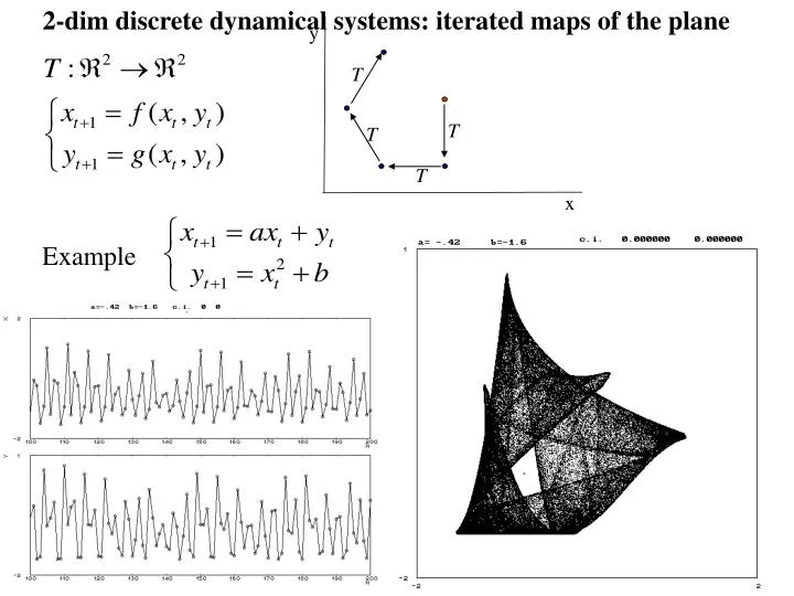
2-dim discrete dynamical systems: iterated maps of the plane. y. T. T. T. T. x. Example. Cournot Duopoly. Two firms produce a homogeneous good and interact in a competitive market, choosing the quantities: q 1 ( t ) e q 2 ( t )

E N D
2-dim discrete dynamical systems: iterated maps of the plane y T T T T x Example
Cournot Duopoly Two firms produce a homogeneous good and interact in a competitive market, choosing the quantities: q1 (t) e q2 (t) Inverse demand function: p = f (q1+q2) = a – b (q1 + q2) Production costs: ci (q1, q2) = ci qi, i = 1,2 Each period profit: Pi= qi f (q1+ q2) – ci (q1, q2) At each stage, they simultaneously decide, solving the problems On the basis of the previous assumptions, we obtain And assuming naive expectations:
Higher order difference equations Example: xt+1 + bxt + cxt-1= 0 With two initial conditions: x0, x1 Let yt = xt-1 Then the difference equation in transformed into: xt+1 = bxtcyt yt+1 = xt
Nonautonomous difference equation. Example. xt+1 = f(xt,t) with i.c. x0 given Let yt = t Then xt+1 = f(xt,yt) yt+1 = yt + 1 with i.c. x0given ; y0 = 0
Linear 2-dim. map Remembering the case of 1-dim linear maps let’s consider the trial solution: And substitute it in the law of evolution: And after dividing by lt we get (A lI) v = lv i.e. the proposed trial is a particular solution provoded that L is an eigenvalue and v is a corresponding eigenvector for the matrix A
Characteristic equation det (AlI) = 0 becomes: P(l) = l2Tr∙l + Det = 0 where Tr = a11+a22 ;Det = a11a22 a12a21 (I) D=Tr24Det >0 then l1 and l2 real and distinct eigenvalues exist with correnponding linearly independent eigenvectors v1, v2, that give rise to two independent soutions and (II) D=0 coincident eigenvalues l, with eigenvector v give two independend solutions ltv and tltv (III) D <0, l1,2= Two independent complex conjugate solutions
Any linear combination of solutions is a solution, hence the generic solution of the linear homogeneous system is; (I) Real and distinct eigenvalues of A, l1 and l2. Denoting by v1 e v2 two eigenvectors respectively associated with them, we obtain (II) Real and equal eigenvalues of A: where c1 and c2 are two suitable vectors dependent on two arbitrary chosen constants (III) Complex conjugated eigenvalues, the real part and the imaginary part of the two independengt complex solutins are solutions,being: where h = h1 + ih2 is an eigenvector associated with l.
Stability of the unique equilibrium: |l|<1 i.e. all eigenvalues inside the unoi circle of the complex plane Iml 1 -1 1 Rel -1 • The origin is an asymptotically stable equilibrium point iff all the eigenvalues are smaller than 1 in modulus. Local stability and global are equivalent • The origin is stable, but not asymptotically, iff the modulus of the eigenvalues is not larger than 1 and all the eigenvalues with unit modulus are regular • Otherwise the origin is unstable
Iml 1 -1 1 Rel Iml Iml Iml Iml Iml 1 1 1 1 1 -1 -1 -1 -1 -1 -1 1 1 1 1 1 Rel Rel Rel Rel Rel -1 -1 -1 -1 -1 STABLE NODE UNSTABLE NODE SADDLE SADDLE UNSTABLE FOCUS STABLE FOCUS
Iml 1 -1 1 Rel -1 • CENTER IMPROPER NODE STAR NODE
Second order • real and distinct eigenvalues: • if |l1| < 1and |l2| < 1 , the origin is globally asymptotically stable (stable node) • if |l1| > 1and |l2| > 1 , the origin is unstable (unstable node) • if |l1| < 1and |l2| > 1 , the origin is unstable (saddle) • equal eigenvalues : • if |l|< 1, the origin is gloablly asymptotically stable (stable node) • if |l|< 1, the origin is unstable (unstable node) • if the matrix A is diagonal: the origin è stable if |l|< 1, unstable if |l|> 1 (star node) • complex conjugated eigenvalues • if r < 1, the origin is globally asymptotically stable (stable focus) • if r > 1 , the origin is unstable (unstable focus) • if r = 1, the origin is stable (center)
Stability triangle unstable node D = Tr24Det=0 1+Tr+Det=0 (Flip curve) 1Tr+Det=0 (Fold curve) unstable focus center if detA = 1, -2<trA<2 Det= 1 (N-S curve) stable focus stable node stable node saddle saddle unstable node center if Det= 1, -2<Tr<2
Cournot Duopoly The model we considered is described by the system of two I^ order linear difference equations The matrix of the system is with distinct real eigenvalues: and the eigenvectors associated with are Solution:
Easily extended to dim >2 • The origin is an asymptotically stable equilibrium point iff all the eigenvalues are smaller than 1 in modulus. Global stability in IRn • The origin is stable, but not asymptotically, iff the modulus of the eigenvalues is not larger than 1 and all the eigenvalues with unit modulus are regular • Otherwise the origin is unstable.
Nonlinear maps of the plane: local stability of a fixed point Let (x*,y*) be a solution of : Linear approximation around (x*,y*) Linear homogeneous system in X = xx* ; Y = yy* Jacobian matrix With
Stability of the equilibrium points • An equilibrium point x* is locally stable if for any neighborhood U of x* there esists a neighborhood VU such that any solution starting in V belongs to U for any t. • If V can be chosen such that x* is said locally asymptotically stable • An equilibrium point is unstable if it is not stable • If x* is an asymptotically stable equilibrium point, the set of the initial condition giving rise to the trajectories converging to x* is the basin of attraction of x* • If the basin of attraction of x* coincides with the whole state space W then x* is globally asymptotically stable.
Local bifurcations in a discrete dynamical system • There are different ways to exit the unit circle: Flip bifurcation (period doubling) Neimark-Sacker bifurcation Fold bifurcation
Bifurcattion lines and the creation of new invariant sets Line of Neimark-Sacker Line of saddle-node Line of flip Where A is the Jacobian matrix computed at the equilibrium considered
An eigenvalue equals to 1 Saddle-Node bifurcation: two fixed points appear, one stable and one unstable Normal form: f(x,a) = a + x-x2
An eigenvalue equals to 1: Pitchfork bifurcation:a fixed point becomes unstable (stable) and two further fixed points appear, both stable (unstable) Normal form:f(x,a) = a x + x-x3 supercritical subcritical
An eigenvalue equals to -1: Flip bifurcation (period doubling bifurcation): • the fixed point becomes unstable and a stable period 2 cycle appears, surrounding it. It corresponds to a pitchfork bifurcation of the second iterated of the map. Normal form:f(x,a) = -(1+a)x + x3 supercritical
Neimark-Sacker bifurcation: The eigenvalues of the Jacobian matrix DT(P*)evaluated at the fixed point P* are complex and cross the unit circle for a = a0. l1 ,k=1,2,3,4 (non resonance conditions) l2 (transversality condition) two alternative situations
P* becomes unstable and an attracting closed curve GS appears around it (supercritical) • P* becomes unstable merging with a repelling closed curve GU,existing • when it is stable (subcritical)
Neimark-Sacker bifurcation:The eigenvalues of the Jacobian matrix DT(P*)evaluated at the fixed point P* are complex and cross the unit circle. ,k=1,2,3,4 (non resonance conditions) (transversality condition) After rescaling P* = 0,ao = 0 nonlinear terms linear terms complex variable: z® l1(a) z + g(z,z,a) z=x1+ix2 change of variable: z=w+h(w) w® m1(a) w + c1w2w + …. r® r(1+ da + ar2 + ….) polar coordinates: w=reib b® b+ q0 + ea + br2 + ….
As the bifurcation parameter moves away from the N-S bifurcation value: The circle slightly deforms, but: • remains an invariant curve • maintains its “stability” • approches a circle for aa0 • Amplitude On the invariant curve: • dense quasiperiodic orbits or • a finite number of periodic orbits, saddles and nodes, appearing and disappearing via Saddle-Node
Arnold tongues inside the Arnold tongues the rotation number is rational m1(a) schematic SN bifurcations bifurcation point (a=ao=0) • Infinitely many tongues, of thickness d (q-2)/2 (d is the distance from the unit circle)
Inside an Arnol’d tongue 1/6 for a stable closed invariant curve (supercritical Neimark-Sacker) Inside an Arnol’d tongue 1/6 for an unstable closed invariant curve (subcritical Neimark-Sacker) Frequency locking: Two cycles appear via Saddle-Node bifurcation The invariant closed curve is given by a saddle-node connection The cycles disappear via Saddle-Node bifurcation.
Example: Iterated map T fixed points: O = (0,0) P = (a,a) Supercritical Neimark-Sacker bifurcation of O occurs at a = 1 O stable focus for a <1 unstable focus for a >1
a = 1.01 a = 1.02 a = 1.05 a = 1.1 a = 1.3 a = 1.4 a = 1.505
T : Rn Rn p’ = T(p) . p1 T . Noninvertible map means “Many-to-One” . p’ p2 T . p1 . T1-1 Equivalently, we say that p’ has several rank-1 preimages . p’ p2 T2-1 Several distinct inverses are defined: i.e. the inverse relation p = T-1(p’) is multivalued Zk LC Rn can be divided into regions (or zones) according to the number of rank-1 preimages Zk+2 Zk: region where k distinct inverses are defined LC (critical manifold): locus of points having two merging preimages
Linear map T : (x,y)→(x’,y’) area (F’) = |det A |area (F), i.e. |det A | < 1 (>1) contraction(expansion) Meaning of the sign of |det A| T is orientation preserving if det A > 0 T is orientation reversing if det A < 0 a11=1 a12=1.5 a21=1 a22 =1 b1= b2= 0; Det = - 0.5 a11=2 a12= -1 a21=1 a22=1 b1= b2= 0 ; Det = 3 y y C C’ C’ C y T T y B’ B’ F F B’ F’ F’ A B B A A’ A’ x x x x
For a continuous map the fold LC-1 is included in the set where det DT(x,y) changes sign in fact, T is orientation preserving near points (x,y) such that det DT(x,y)>0 orientation reversing if det DT(x,y) < 0 If T is continuously differentiable LC-1 is included in the set where det DT(x,y) = 0 The critical set LC = T ( LC-1 )
A noninvertible map of the plane “folds and pleats”' the plane so that distinct points are mapped into the same point. T LC-1 LC = T(LC-1) R2 R1 Z2 Z0 SH1 SH2 LC-1 LC Z2 Z0 R2 R1 Riemann Foliation A point has several distinct preimages, i.e. several inverses are defined in it, which “unfold” the plane A region Zk is seen as the superposition of k sheets, each associated with a different inverse, connected by folds along LC
fixed points: O = (0,0) P = (l,l) Example: LC = {(x,y) | y = x –l2/4} LC-1 = {(x,y) | x = l/2 } Z2 = {(x,y) | y > x– l2/4} Z0 = {(x,y) | y < x– l2/4 y < b } det DT = a 2x = 0 for x = l/2 T({x = a/2 }) = {y = x –a2/4} Supercritical Neimark-Sacker bif. at a = 1
P LC Z2 Z0 G O R1 R2 LC-1
P LC-1 A0 Z2 LC G Z0 A1 B0 O h1 R1 R2 B1
C1 C7 G C2 LC C3 O C6 C4 LC-1 C5
P LC O LC-1
P O
Mappa non invertibile y a = 1 b = -2 y . . . . 3 3 P = T(P1) = T(P2) 2 2 P . . 1 1 x x -3 -2 1 3 2 -1 -3 -2 1 3 2 -1 -1 -1 -2 -2 2 inverse
det DT = -2x =0 for x=0 T({x=0}) = {y=b} LC = {(x,y) | y = b } LC-1 = {(x,y) | x = 0 } Z2 = {(x,y) | y > b } Z0 = {(x,y) | y < b } R1 SH1 R2 SH2 LC-1 Z2 y=b LC x=0 Z0
T: T F F’= T(F) LC -1 LC
LC-1 LC-1 y y C D C B A B A O B’ C’ A’ B’ A’ D’ LC LC C’ O’ x x LC-1 LC-1 y B y B A C C A C’ B’ C’ B’ A’ A’ LC LC x x (b) (a)
LC 2 LC 5 LC 6 LC 1 LC LC -1 LC 3 4 LC f: