Download
1 / 78
780 likes | 835 Views
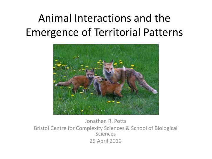
Animal Interactions and the Emergence of Territorial Patterns. Jonathan R. Potts Bristol Centre for Complexity Sciences & School of Biological Sciences 29 April 2010. Outline. Outline.

E N D
Animal Interactions and the Emergence of Territorial Patterns Jonathan R. Potts Bristol Centre for Complexity Sciences & School of Biological Sciences 29 April 2010
Outline • Introduce the main problem: how territorial and home-range patterns emerge from animal movements and interactions
Outline • Introduce the main problem: how territorial and home-range patterns emerge from animal movements and interactions • Describe a model we’ve built to tackle this problem
Outline • Introduce the main problem: how territorial and home-range patterns emerge from animal movements and interactions • Describe a model we’ve built to tackle this problem • Results and analysis of the model
Outline • Introduce the main problem: how territorial and home-range patterns emerge from animal movements and interactions • Describe a model we’ve built to tackle this problem • Results and analysis of the model • Application to data set on the red fox (Vulpesvulpes)
Outline • Introduce the main problem: how territorial and home-range patterns emerge from animal movements and interactions • Describe a model we’ve built to tackle this problem • Results and analysis of the model • Application to data set on the red fox (Vulpesvulpes) • Questions
How do home range and territory patterns emerge? • Definitions: • An animal’s home range (HR) is the area in which it spends it’s time during “everyday” activities. • An animal’s territory is a defended area from which conspecifics are excluded.
How do home range and territory patterns emerge? • Definitions: • An animal’s home range (HR) is the area in which it spends it’s time during “everyday” activities. • An animal’s territory is a defended area from which conspecifics are excluded. • Idea: They must both emerge somehow from the movements and interactions of the animals.
How do home range and territory patterns emerge? • Definitions: • An animal’s home range (HR) is the area in which it spends it’s time during “everyday” activities. • An animal’s territory is a defended area from which conspecifics are excluded. • Idea: They must both emerge somehow from the movements and interactions of the animals. • Question: How does this happen?
How do home range and territory patterns emerge? • Definitions: • An animal’s home range (HR) is the area in which it spends it’s time during “everyday” activities. • An animal’s territory is a defended area from which conspecifics are excluded. • Idea: They must both emerge somehow from the movements and interactions of the animals. • Question: How does this happen? • Approach: • Build a model using features of the animals’ movements and interactions. • See which features are important by analysing the model’s output against HR patterns from the data.
The red fox: a model example • Our model is based on the behaviour of the urban red fox (Vulpesvulpes). • Over 30 years of movement data in Bristol (collected by Steve Harris and co-workers).
The red fox: a model example • Our model is based on the behaviour of the urban red fox (Vulpesvulpes). • Over 30 years of movement data in Bristol (collected by Steve Harris and co-workers). • Key features used in model: • Hinterland marker. Scents homogeneously as it moves. • Conspecific avoidance. On encountering the scent of a neighbour, the animal does not advance into the neighbouring territory.
The red fox: a model example • Our model is based on the behaviour of the urban red fox (Vulpesvulpes). • Over 30 years of movement data in Bristol (collected by Steve Harris and co-workers). • Key features used in model: • Hinterland marker. Scents homogeneously as it moves. • Conspecific avoidance. On encountering the scent of a neighbour, the animal does not advance into the neighbouring territory. • The model can be applied to any animal with these two behavioural features.
The model • Individuals exist in a lattice with periodic boundary conditions.
The model • Individuals exist in a lattice with periodic boundary conditions.
The model • Individuals exist in a lattice with periodic boundary conditions. • They deposit scent at every site they visit.
The model • Individuals exist in a lattice with periodic boundary conditions. • They deposit scent at every site they visit. • Scent remains for a fixed number of timesteps: the Active Scent Time,TAS.
The model • Individuals exist in a lattice with periodic boundary conditions. • They deposit scent at every site they visit. • Scent remains for a fixed number of timesteps: the Active Scent Time,TAS. • If an individual is at a lattice site that does not contain foreign scent then it moves to a neighbouring lattice site at random.
The model • Individuals exist in a lattice with periodic boundary conditions. • They deposit scent at every site they visit. • Scent remains for a fixed number of timesteps: the Active Scent Time,TAS. • If an individual is at a lattice site that does not contain foreign scent then it moves to a neighbouring lattice site at random. • If an individual is at a lattice site that does contain foreign scent then it moves to a neighbouring lattice site that does not contain foreign scent (chosen at random).
Model output – position density plots • Left plot: the position densities of 8 animals after running the 2D simulation. • Additional feature: Boundary-dependent correlation (BDC). The random walk changes to a correlated RW after reaching the territory boundary. This correlation decays as the walker moves away. • Top right: 1D walkers with no BDC. • Below: 1D walkers withBDC.
Quantifying the relationship between territories and home ranges
Quantifying the relationship between territories and home ranges • To quantify this relation, we look at the movement of the territoryboundaries (for which we use the 1D model).
Quantifying the relationship between territories and home ranges • To quantify this relation, we look at the movement of the territoryboundaries (for which we use the 1D model). • The boundaries obey a single file diffusion process.
Quantifying the relationship between territories and home ranges • To quantify this relation, we look at the movement of the territoryboundaries (for which we use the 1D model). • The boundaries obey a single file diffusion process. • Well understood in physics literature.
Quantifying the relationship between territories and home ranges • To quantify this relation, we look at the movement of the territoryboundaries (for which we use the 1D model). • The boundaries obey a single file diffusion process. • Well understood in physics literature. • Random walker, constrained by nearby random walkers.
Quantifying the relationship between territories and home ranges • To quantify this relation, we look at the movement of the territoryboundaries (for which we use the 1D model). • The boundaries obey a single file diffusion process. • Well understood in physics literature. • Key features: • The mean square displacement (MSD) scales asymptotically as t1/2 (MSD = variance of the probability distribution) so that, at long times where b(t) is the position of the boundary, k is a type of “(sub)-diffusion constant”, dependent on TAS and the population density, ρ.
Quantifying the relationship between territories and home ranges • To quantify this relation, we look at the movement of the territoryboundaries (for which we use the 1D model). • The boundaries obey a single file diffusion process. • Well understood in physics literature. • Key features: • The mean square displacement (MSD) scales asymptotically as t1/2 (MSD = variance of the probability distribution) so that, at long times where b(t) is the position of the boundary, k is a type of “(sub)-diffusion constant”, dependent on TAS and the population density, ρ.
Quantifying the relationship between territories and home ranges • To quantify this relation, we look at the movement of the territoryboundaries (for which we use the 1D model). • The boundaries obey a single file diffusion process. • Well understood in physics literature. • Key features: • The mean square displacement (MSD) scales asymptotically as t1/2 (MSD = variance of the probability distribution) so that, at long times where b(t) is the position of the boundary, k is a type of “(sub)-diffusion constant”, dependent on TAS and the population density, ρ. displacement
Quantifying the relationship between territories and home ranges • To quantify this relation, we look at the movement of the territoryboundaries (for which we use the 1D model). • The boundaries obey a single file diffusion process. • Well understood in physics literature. • Key features: • The mean square displacement (MSD) scales asymptotically as t1/2 (MSD = variance of the probability distribution) so that, at long times where b(t) is the position of the boundary, k is a type of “(sub)-diffusion constant”, dependent on TAS and the population density, ρ. square displacement
Quantifying the relationship between territories and home ranges • To quantify this relation, we look at the movement of the territoryboundaries (for which we use the 1D model). • The boundaries obey a single file diffusion process. • Well understood in physics literature. • Key features: • The mean square displacement (MSD) scales asymptotically as t1/2 (MSD = variance of the probability distribution) so that, at long times where b(t) is the position of the boundary, k is a type of “(sub)-diffusion constant”, dependent on TAS and the population density, ρ. mean square displacement
Quantifying the relationship between territories and home ranges • To quantify this relation, we look at the movement of the territoryboundaries (for which we use the 1D model). • The boundaries obey a single file diffusion process. • Well understood in physics literature. • Key features: • The mean square displacement (MSD) scales asymptotically as t1/2 (MSD = variance of the probability distribution) so that, at long times where b(t) is the position of the boundary, k is a type of “(sub)-diffusion constant”, dependent on TAS and the population density, ρ. mean square displacement time
Quantifying the relationship between territories and home ranges • To quantify this relation, we look at the movement of the territoryboundaries (for which we use the 1D model). • The boundaries obey a single file diffusion process. • Well understood in physics literature. • Key features: • The mean square displacement (MSD) scales asymptotically as t1/2 (MSD = variance of the probability distribution) so that, at long times where b(t) is the position of the boundary, k is a type of “(sub)-diffusion constant”, dependent on TAS and the population density, ρ. • The probability distribution is Gaussian (a.k.a. Normal), which means that the X% Minimum Convex Polygon (MCP) can be derived from the MSD of the distribution (e.g. if X=90, the width of 90% MCP of the boundary is 1.645*2*MSD1/2).
Quantifying the relationship between territories and home ranges • To quantify this relation, we look at the movement of the territoryboundaries (for which we use the 1D model). • The boundaries obey a single file diffusion process. • Well understood in physics literature. • Key features: • The mean square displacement (MSD) scales asymptotically as t1/2 (MSD = variance of the probability distribution) so that, at long times where b(t) is the position of the boundary, k is a type of “(sub)-diffusion constant”, dependent on TASand the population density, ρ. • The probability distribution is Gaussian (a.k.a. Normal), which means that the X% Minimum Convex Polygon (MCP) can be derived from the MSD of the distribution (e.g. if X=90, the width of 90% MCP of the boundary is 1.645*2*MSD1/2). Key quantity to understand
Quantifying the boundary movement • The value of k decreases exponentially with the product of TAS and ρ2.
Quantifying the boundary movement • The value of k decreases exponentially with the product of TAS and ρ2. • TAS↔k ↔ distribution of b(t) ↔ boundary MCP ↔ HR size and overlaps
Quantifying the boundary movement • The value of k decreases exponentially with the product of TAS and ρ2. • TAS↔k ↔ distribution of b(t) ↔ boundary MCP ↔ HR size and overlaps • Why the product of ρ2 and TAS?
Quantifying the boundary movement • The value of k decreases exponentially with the product of TAS and ρ2. • TAS↔k ↔ distribution of b(t) ↔ boundary MCP ↔ HR size and overlaps • Why the product of ρ2 and TAS? • For large TAS, it turns out that ρ2 is approximately 1/TFP, where TFP is the time it takes, on average, for the individual to go from one boundary to the other (the first-passage time).
Quantifying the boundary movement Territory • The value of k decreases exponentially with the product of TAS and ρ2. • TAS↔k ↔ distribution of b(t) ↔ boundary MCP ↔ HR size and overlaps • Why the product of ρ2 and TAS? • For large TAS, it turns out that ρ2 is approximately 1/TFP, where TFP is the time it takes, on average, for the individual to go from one boundary to the other (the first-passage time).
Quantifying the boundary movement Territory scent • The value of k decreases exponentially with the product of TAS and ρ2. • TAS↔k ↔ distribution of b(t) ↔ boundary MCP ↔ HR size and overlaps • Why the product of ρ2 and TAS? • For large TAS, it turns out that ρ2 is approximately 1/TFP, where TFP is the time it takes, on average, for the individual to go from one boundary to the other (the first-passage time).
Quantifying the boundary movement Territory scent • The value of k decreases exponentially with the product of TAS and ρ2. • TAS↔k ↔ distribution of b(t) ↔ boundary MCP ↔ HR size and overlaps • Why the product of ρ2 and TAS? • For large TAS, it turns out that ρ2 is approximately 1/TFP, where TFP is the time it takes, on average, for the individual to go from one boundary to the other (the first-passage time).
Quantifying the boundary movement Territory scent • The value of k decreases exponentially with the product of TAS and ρ2. • TAS↔k ↔ distribution of b(t) ↔ boundary MCP ↔ HR size and overlaps • Why the product of ρ2 and TAS? • For large TAS, it turns out that ρ2 is approximately 1/TFP, where TFP is the time it takes, on average, for the individual to go from one boundary to the other (the first-passage time).
Quantifying the boundary movement Territory scent • The value of k decreases exponentially with the product of TAS and ρ2. • TAS↔k ↔ distribution of b(t) ↔ boundary MCP ↔ HR size and overlaps • Why the product of ρ2 and TAS? • For large TAS, it turns out that ρ2 is approximately 1/TFP, where TFP is the time it takes, on average, for the individual to go from one boundary to the other (the first-passage time).
Quantifying the boundary movement Territory scent • The value of k decreases exponentially with the product of TAS and ρ2. • TAS↔k ↔ distribution of b(t) ↔ boundary MCP ↔ HR size and overlaps • Why the product of ρ2 and TAS? • For large TAS, it turns out that ρ2 is approximately 1/TFP, where TFP is the time it takes, on average, for the individual to go from one boundary to the other (the first-passage time).
Quantifying the boundary movement Territory scent • The value of k decreases exponentially with the product of TAS and ρ2. • TAS↔k ↔ distribution of b(t) ↔ boundary MCP ↔ HR size and overlaps • Why the product of ρ2 and TAS? • For large TAS, it turns out that ρ2 is approximately 1/TFP, where TFP is the time it takes, on average, for the individual to go from one boundary to the other (the first-passage time).