Download
1 / 62
620 likes | 878 Views
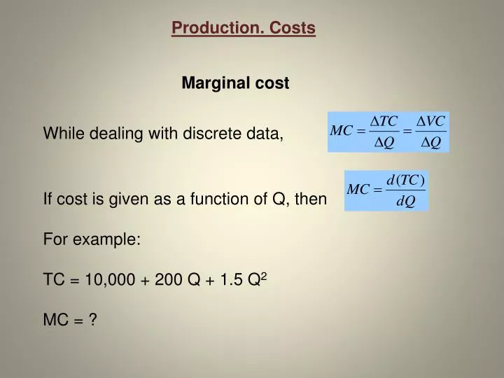
Production. Costs. Marginal cost. While dealing with discrete data,. If cost is given as a function of Q, then For example: TC = 10,000 + 200 Q + 1.5 Q 2 MC = ?. Problem 2 on p.194. “Diminishing returns” – what are they?.

E N D
Production. Costs Marginal cost While dealing with discrete data, If cost is given as a function of Q, then For example: TC = 10,000 + 200 Q + 1.5 Q2 MC = ?
Problem 2 on p.194. “Diminishing returns” – what are they? In the short run, every company has some inputs fixed and some variable. As the variable input is added, every extra unit of that input increases the total output by a certain amount; this additional amount is called “marginal product”. The term, diminishing returns, refers to the situation when the marginal product of the variable input starts to decrease (even though the total output may still keep going up!)
Total output, or Total Product, TP Amount of input used Range of diminishing returns Marginal product, MP Amount of input used
Calculating the marginal product (of capital) for the data in Problem 2:
Calculating the marginal product (of capital) for the data in Problem 2:
Calculating the marginal product (of capital) for the data in Problem 2:
In other words, we know we are in the range of diminishing returns when the marginal product of the variable input starts falling, or, the rate of increase in total output slows down. (Ex: An extra worker is not as useful as the one before him) Implications for the marginal cost relationship: Worker #10 costs $8/hr, makes 10 units. MCunit =
In other words, we know we are in the range of diminishing returns when the marginal product of the variable input starts falling, or, the rate of increase in total output slows down. (Ex: An extra worker is not as useful as the one before him) Implications for the marginal cost relationship: • Worker #10 costs $8/hr, makes 10 units. MCunit = $0.80 Worker #11 costs $8/hr, makes …
In other words, we know we are in the range of diminishing returns when the marginal product of the variable input starts falling, or, the rate of increase in total output slows down. (Ex: An extra worker is not as useful as the one before him) Implications for the marginal cost relationship: • Worker #10 costs $8/hr, makes 10 units. MCunit = $0.80 Worker #11 costs $8/hr, makes 8 units. MCunit =
In other words, we know we are in the range of diminishing returns when the marginal product of the variable input starts falling, or, the rate of increase in total output slows down. (Ex: An extra worker is not as useful as the one before him) Implications for the marginal cost relationship: • Worker #10 costs $8/hr, makes 10 units. MCunit = $0.80 Worker #11 costs $8/hr, makes 8 units. MCunit = $1 In the range of diminishing returns, MP of input is falling and MC of output is increasing
Marginal cost, MC Amount of output This amount of output corresponds to thisamount of input Marginal product, MP Amount of input used
When MP of input is decreasing, MC of output is increasing and vice versa. Therefore the range of diminishing returns can be identified by looking at either of the two graphs. (Diminishing marginal returns set in at the max of the MP graph, or at the min of the MC graph)
Profit is believed to be the ultimate goal of any firm. In Problem 2, what number of units of capital maximizes the firm’s profit? PK = $75 PL = $15 POUTPUT = $2 The aggregate approach:
Profit is believed to be the ultimate goal of any firm. In Problem 2, what number of units of capital maximizes the firm’s profit? PK = $75 PL = $15 POUTPUT = $2 The aggregate approach:
Profit is believed to be the ultimate goal of any firm. In Problem 2, what number of units of capital maximizes the firm’s profit? PK = $75 PL = $15 POUTPUT = $2 The aggregate approach:
Profit is believed to be the ultimate goal of any firm. In Problem 2, what number of units of capital maximizes the firm’s profit? PK = $75 PL = $15 POUTPUT = $2 The aggregate approach:
Principle (Marginal approach to profit maximization): • If data is provided in discrete (tabular) form, then profit is maximized by producing all the units for which and stopping right before the unit for which
Principle (Marginal approach to profit maximization): • If data is provided in discrete (tabular) form, then profit is maximized by producing all the units for which MR > MCand stopping right before the unit for which MR < MC • In our case, price of output stays constant throughout therefore MR = P • (an extra unit increases TR by the amount it sells for) • If costs are continuous functions of QOUTPUT, then profit is maximized where
Principle (Marginal approach to profit maximization): • If data is provided in discrete (tabular) form, then profit is maximized by producing all the units for which MR > MCand stopping right before the unit for which MR < MC • In our case, price of output stays constant throughout therefore MR = P • (an extra unit increases TR by the amount it sells for) • If costs are continuous functions of QOUTPUT, then profit is maximized where MR=MC
The marginal approach: To find the profit maximizing amount of input (part d), we need to compare the marginal benefit from a change to the marginal cost of than change. More specifically, we compare VMPK, the value of marginal product of capital, to the price of capital, or the “rental rate”, r.
Back to problem 2, p.194. To find the profit maximizing amount of input (part d), we will once again use the marginal approach, which compares the marginal benefit from a change to the marginal cost of than change. More specifically, we compare VMPK, the value of marginal product of capital, to the price of capital, or the “rental rate”, r.
Back to problem 2, p.194. To find the profit maximizing amount of input (part d), we will once again use the marginal approach, which compares the marginal benefit from a change to the marginal cost of than change. More specifically, we compare VMPK, the value of marginal product of capital, to the price of capital, or the “rental rate”, r. > > > > > STOP <
Back to problem 2, p.194. To find the profit maximizing amount of input (part d), we will once again use the marginal approach, which compares the marginal benefit from a change to the marginal cost of than change. More specifically, we compare VMPK, the value of marginal product of capital, to the price of capital, or the “rental rate”, r. > > > > > STOP <
What if the cost of labor (the fixed cost in this case) changes? How does the profit maximization point change?
What if the cost of labor (the fixed cost in this case) changes? How does the profit maximization point change?
What if the cost of labor (the fixed cost in this case) changes? How does the profit maximization point change?
Principle: Fixed cost does not affect the firm’s optimal short-term output decision and can be ignored while deciding how much to produce today. Consistently low profits may induce the firm to close down eventually (in the long run) but not any sooner than your fixed inputs become variable ( your building lease expires, your equipment wears out and new equipment needs to be purchased, you are facing the decision of whether or not to take out a new loan, etc.)
Why would we ever want to be in the range of diminishing returns? Consider the simplest case when the price of output doesn’t depend on how much we produce. Until we get to the DMR range, every next worker is more valuable than the previous one, therefore we should keep hiring them. Only afterwe get to the DMR range and the MP starts falling, we should consider stopping. Therefore, the profit maximizing point is always in the diminishing marginal returns range! Surprised?
Cost minimization (Another important aspect of being efficient.) Suppose that, contrary to the statement of the last problem, we ARE ABLE to change not just the amount of capital but the amount of labor as well. (Recall the distinction between the long run and the short run.) Given that extra degree of freedom, can we do better? (In other words, is there a better way to allocate our budget to achieve our production goals?)
In order not to get lost in the multiple possible (K, L, Q) combinations, it is useful to have some of them fixed and focus on the question of interest. • In our case, we can either: • Fix the total budget spent on inputs and see if we can increase the total output; • or, • Fix the target output and see if we can reduce the total cost by spending our money differently.
Think of the following analogy: Sam needs his 240 mg of caffeine a day or he will fall asleep while driving, and something bad will happen. He can get his caffeine fix from several options listed below: Which one should he choose?
Think of the following analogy: Sam needs his 240 mg of caffeine a day or he will fall asleep while driving, and something bad will happen. He can get his caffeine fix from several options listed below:
Think of the following analogy: Sam needs his 240 mg of caffeine a day or he will fall asleep while driving, and something bad will happen. He can get his caffeine fix from several options listed below:
Think of the following analogy: Sam needs his 240 mg of caffeine a day or he will fall asleep while driving, and something bad will happen. He can get his caffeine fix from several options listed below:
Think of the following analogy: Sam needs his 240 mg of caffeine a day or he will fall asleep while driving, and something bad will happen. He can get his caffeine fix from several options listed below:
Think of the following analogy: Sam needs his 240 mg of caffeine a day or he will fall asleep while driving, and something bad will happen. He can get his caffeine fix from several options listed below:
Next, think of caffeine as Sam’s ‘target output’ (what he is trying to achieve)and drinks as his inputs, which can to a certain extent be substituted for each other. The same principle holds for any production unit that is trying to allocate its resources wisely: In order to achieve the most at the lowest cost possible, a firm should go with the option with the highest MPinput/Pinputratio. Note that following this principle will make the firm better off regardless of the demand it is facing!
If then - reduce the amount of capital; - increase the amount of labor. • As you do that, • MPL will decrease; • MPC will increase; • the LHS will get smaller, • the RHS bigger If then - reduce the amount of labor; - increase the amount of capital. If then inputs are used in the right proportion. No need to change anything.
Profit maximization in different market structures In the Elasticity topic, we discussed a firm facing downward-sloping demand – if a company wants to attract more customers, it has to lower its price. Tonight,we considered examples where the price the firm could get for each unit of out put did not depend on the number of units produced. Which way is right? Which way is more realistic therefore more relevant?
Traditionally, economics textbooks distinguish four types of markets, or of market structures. They differ in the degree of market power an individual firm has: • Perfect competition • Monopolistic competition • Oligopoly • Monopoly the least market power the most market power • “Market power” also known as “pricing power” is defined in the managerial literature as the ability of an individual firm to vary its price while still remaining profitableor as • the firm’s ability to charge the price above its MC.
Perfect competition The features of a perfectly competitive market are: • Large number of competing firms; • Firms are small relative to the entire market; • Products different firms make are identical; • Information on prices is readily available.
As a result, the price is set by the interaction of supply and demand forces, and an individual firm can do nothing about the price. P Q This is the story of any small-size firm that cannot differentiate itself from the others.
What does a Total Revenue (TR) graph look like for such a firm, if plotted against quantity produced/sold? TR Every unit sells at the same price so… Slope equals price Q
How about the Marginal Revenue graph? MR Every unit sells at the same price so… MR = P Q
The profit maximization story told graphically: In aggregate terms: TC TR Profit FC Q max capacity max profit
In marginal terms: MC MR Q max profit
Doing the same thing mathematically: TC = 100 + 40 Q + 5 Q2 , And the market price is $160, What is the profit maximizing quantity (remember, price is determined by the market therefore it is given)? Just like in the case with tabular data, there are two approaches.
Aggregate: • Profit = TR – TC =
Aggregate: • Profit = TR – TC = 160 Q – (100 + 40 Q + 5 Q2)
Aggregate: • Profit = TR – TC = 160 Q – (100 + 40 Q + 5 Q2) = • =120 Q – 100 – 5 Q2 A function is maximized when its derivative is zero; Specifically, when it changes its sign from ( + ) to ( – ) • d(Profit)/dQ = 0 • 120 – 10 Q = 0 • Q = 12