Download
1 / 55
550 likes | 707 Views
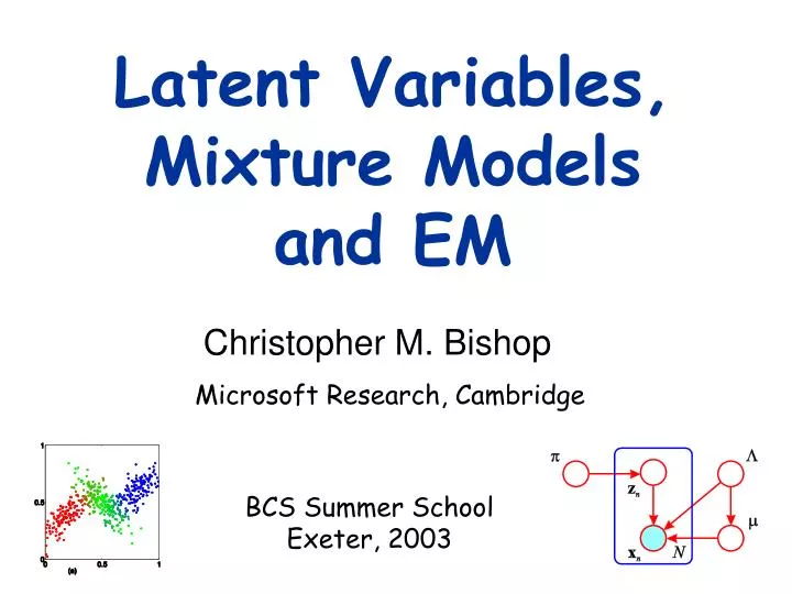
Latent Variables, Mixture Models and EM. Christopher M. Bishop. Microsoft Research, Cambridge. BCS Summer School Exeter, 2003. Overview. K-means clustering Gaussian mixtures Maximum likelihood and EM Latent variables: EM revisited Bayesian Mixtures of Gaussians. Old Faithful.

E N D
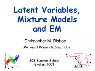
Latent Variables,Mixture Modelsand EM Christopher M. Bishop Microsoft Research, Cambridge BCS Summer SchoolExeter, 2003
Overview. • K-means clustering • Gaussian mixtures • Maximum likelihood and EM • Latent variables: EM revisited • Bayesian Mixtures of Gaussians
Old Faithful Data Set Time betweeneruptions (minutes) Duration of eruption (minutes)
K-means Algorithm • Goal: represent a data set in terms of K clusters each of which is summarized by a prototype • Initialize prototypes, then iterate between two phases: • E-step: assign each data point to nearest prototype • M-step: update prototypes to be the cluster means • Simplest version is based on Euclidean distance • re-scale Old Faithful data
Responsibilities • Responsibilities assign data points to clusterssuch that • Example: 5 data points and 3 clusters
data prototypes responsibilities K-means Cost Function
Minimizing the Cost Function • E-step: minimize w.r.t. • assigns each data point to nearest prototype • M-step: minimize w.r.t • gives • each prototype set to the mean of points in that cluster • Convergence guaranteed since there is a finite number of possible settings for the responsibilities
Limitations of K-means • Hard assignments of data points to clusters – small shift of a data point can flip it to a different cluster • Not clear how to choose the value of K • Solution: replace ‘hard’ clustering of K-means with ‘soft’ probabilistic assignments • Represents the probability distribution of the data as a Gaussian mixture model
covariance mean The Gaussian Distribution • Multivariate Gaussian • Define precision to be the inverse of the covariance • In 1-dimension
Likelihood Function • Data set • Assume observed data points generated independently • Viewed as a function of the parameters, this is known as the likelihood function
Maximum Likelihood • Set the parameters by maximizing the likelihood function • Equivalently maximize the log likelihood
Maximum Likelihood Solution • Maximizing w.r.t. the mean gives the sample mean • Maximizing w.r.t covariance gives the sample covariance
Gaussian Mixtures • Linear super-position of Gaussians • Normalization and positivity require • Can interpret the mixing coefficients as prior probabilities
Sampling from the Gaussian • To generate a data point: • first pick one of the components with probability • then draw a sample from that component • Repeat these two steps for each new data point
Fitting the Gaussian Mixture • We wish to invert this process – given the data set, find the corresponding parameters: • mixing coefficients • means • covariances • If we knew which component generated each data point, the maximum likelihood solution would involve fitting each component to the corresponding cluster • Problem: the data set is unlabelled • We shall refer to the labels as latent (= hidden) variables
Posterior Probabilities • We can think of the mixing coefficients as prior probabilities for the components • For a given value of we can evaluate the corresponding posterior probabilities, called responsibilities • These are given from Bayes’ theorem by
Maximum Likelihood for the GMM • The log likelihood function takes the form • Note: sum over components appears inside the log • There is no closed form solution for maximum likelihood
Problems and Solutions • How to maximize the log likelihood • solved by expectation-maximization (EM) algorithm • How to avoid singularities in the likelihood function • solved by a Bayesian treatment • How to choose number K of components • also solved by a Bayesian treatment
EM Algorithm – Informal Derivation • Let us proceed by simply differentiating the log likelihood • Setting derivative with respect to equal to zero givesgivingwhich is simply the weighted mean of the data
EM Algorithm – Informal Derivation • Similarly for the covariances • For mixing coefficients use a Lagrange multiplier to give
EM Algorithm – Informal Derivation • The solutions are not closed form since they are coupled • Suggests an iterative scheme for solving them: • Make initial guesses for the parameters • Alternate between the following two stages: • E-step: evaluate responsibilities • M-step: update parameters using ML results
EM – Latent Variable Viewpoint • Binary latent variables describing which component generated each data point • Conditional distribution of observed variable • Prior distribution of latent variables • Marginalizing over the latent variables we obtain
Expected Value of Latent Variable • From Bayes’ theorem
Complete and Incomplete Data complete incomplete
Latent Variable View of EM • If we knew the values for the latent variables, we would maximize the complete-data log likelihoodwhich gives a trivial closed-form solution (fit each component to the corresponding set of data points) • We don’t know the values of the latent variables • However, for given parameter values we can compute the expected values of the latent variables
Expected Complete-Data Log Likelihood • Suppose we make a guess for the parameter values (means, covariances and mixing coefficients) • Use these to evaluate the responsibilities • Consider expected complete-data log likelihood where responsibilities are computed using • We are implicitly ‘filling in’ latent variables with best guess • Keeping the responsibilities fixed and maximizing with respect to the parameters give the previous results