Download
1 / 24
240 likes | 424 Views
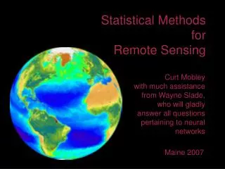
Statistical Methods for Remote Sensing. Curt Mobley with much assistance from Wayne Slade, who will gladly answer all questions pertaining to neural networks. Maine 2007. Inverse Problems.

E N D
Statistical MethodsforRemote Sensing Curt Mobley with much assistance from Wayne Slade, who will gladly answer all questions pertaining to neural networks Maine 2007
Inverse Problems Forward problems usually have a unique solution. For example, you put the IOPs and boundary conditions into the the RTE, and there is only one corresponding radiance distribution. Inverse problems may have a unique solution in principle (e.g., if you have complete and noise-free data), but they seldom have a unique solution in practice (e.g., if you have incomplete or noisy data). For example, there may be more than one set of IOPs that give the same Rrs within the error of the Rrs measurement. Unfortunately, remote sensing is an inverse problem.
Statistical Methods • Statistical (aka empirical) methods: • first assume a mathematical model that relates the known quantities (usually Rrs; the model input) to the unknown quantities (Chl, TSM, a, bb, Kd, bottom depth, etc.; the model output) • then use data to determine the values of the model parameters (weighting functions, best-fit coefficients) • After the parameters are determined, you can feed new input to the model to estimate the quantities of interest. • Two examples: • band-ratio algorithm • neural networks
443 520 550 670 Where It All Started The seminal idea of ocean color remote sensing: Chl concentration and water-leaving radiance are correlated.
R(1,3) = Lw(1=443)/Lw(3=550) vs Chl Note: only 33 data points were initially available! Suggests the band-ratio model: log10(Chl) = C1 + C2log10 [Lw(443)/Lw(550)] C1 and C2 are the model parameters whose values are determined by the data
CZCS Image Coastal Zone Color Scanner (CZCS) 1978-1986 4 visible, 2 IR bands 66,000 images revolutionized oceanography with very simple band ratio algorithms Chl = 0.2 in blue to 30 in red
Examples of Recent Band-Ratio Algorithms • SeaWiFS OC4v4 for Chl: • X = log10{max[Rrs(443)/Rrs(555), Rrs(490)/Rrs(555), Rrs(510)/Rrs(555)]} • Chl = 10^(0.366 - 3.067X + 1.930X2 + 0.649X3 - 1.532X4) • MODIS for Kd(490): • X = Lw(488)/Lw(551) • Kd(490) = 0.016 + 0.156445X^(-1.5401) • MODIS for aCDOM(400) and aphy(675): • r15 = log10[Rrs(412)/Rrs(551)] • r25 = log10[Rrs(443)/Rrs(551)] • r35 = log10[Rrs(488)/Rrs(551)] • aCDOM(400) = 1.5*10^(-1.147 + 1.963r15 - 1.01r152 - 0.856r25 + 1.02r252) • aphy(675) = 0.328 [ 10^(-0.919 + 1.037r25 - 0.407r252 - • 3.531r35 + 1.702r352 - 0.008)] • and so on, for dozens more….
A Fun Project Use Hydrolight to generate some Rrs spectra for various case 1 and case 2 IOPs. Then run these Rrs through various band-ratio algorithms to see how the retrieved values compare with each other and with what went into Hydrolight. This page of retrieval algorithms is on z:\BandRatioAlgorithms.gif You can find more on the www. MODIS Chl Case 1 MODIS Kd(490) MODIS Chl Case 2 MODIS Chl Case 2 MODIS a(675) & aCDOM(400) CZCS Chl SeaWiFS Chl
Nonuniqueness Band-ratio algorithms are vulnerable to non-uniqueness problems because the Rrs ratioing throws out magnitude information that makes spectra unique. Every spectrum below has Rrs(490)/Rrs(555) = 1.710.01, which gives Chl = 0.59 mg/m3 by the SeaWiFS OC2 algorithm; all of these spectra had Chl < 0.2 mg/m3.
O’Reilly et al., JGR, 1998 Model Selection In some situations, you can figure out (from intuition, theoretical guidance, or data analysis) the general mathematical form of the model that links the input and output (e.g., the polynomial functions that relate the band ratios to Chl). You can then use the available data (e.g., simultaneous measurements of Rrs() and Chl) to get best-fit coefficients in the model via least-squares fitting. But what if you don’t have a clue what the mathematical form of the model is?
Neural Networks • Neural networks are a form of multiprocessor computation, based on the parallel architecture of animal brains, with • simple processing elements • a high degree of connection between elements • simple input and output (real numbers) • adaptive interaction between elements • Neural networks are useful • where we don’t know the mathematical form of the model linking the input and output • where we have lots of examples of the behavior we require (lots of data to “train” the NN) • where we need to determine the model structure from the existing data
inputs processing outputs stolen from www.qub.ac.uk/mgt/intsys/nnbiol.html Biological Neural Networks
w1 If x1w1 + x2w2 + b < t output = 0, else output = 1 x1 Output w2 x2 A Simple Artificial Neural Network input layer synaptic weights hidden layer (neurons) output layer In the neuron, b is the bias, t is the threshhold value • The neuron (processor) does two simple things: • (1) it sums the weighted inputs • (2) compares the biased sum to a threshhold value to • determine its output
Training the Neural Network (1) The essence of a neural network is that it can learn from available data. This is called training the NN. The NN has to learn what weighting functions will generate the desired output from the input. Training can be done by backpropagation of errors when known inputs are compared with known outputs. We feed the NN various inputs along with the correct outputs, and let the NN objectively adjust its weights until it can reproduce the desired outputs. The Java applet at www.qub.ac.uk/mgt/intsys/perceptr.html illustrates how a simple NN is trained by backpropagation.
Things to Note The NN was able to use the training data to determine a set of weights so that the given input produced the desired output. After training, we hope (in more complex networks) that new inputs (not in the training data set) will also produce correct outputs. The “knowledge” or “memory” of a neural network is contained in the weights. In a more complicated situation, you must balance having enough neurons to capture the science, but not so many that the network learns the noise in the training data.
Training the Neural Network (2) Another way to train a NN is to view the NN as a complicated mathematical model that connects the inputs and outputs via equations whose coefficients (the weights) are unknown. Then use a non-linear least squares fitting/search algorithm (e.g., Levenberg-Marquardt) to find the “best fit” set of weights for the given inputs and outputs (the training data). This makes is clear that NNs are just fancy regression models whose coefficients/weights are determined by fancy curve fitting to the available data (not a criticism!)
An Example NN • From Ressom, H., R. L. Miller, P. Natarajan, and W. H. Slade, 1995. Computational Intelligence and its Application in Remote Sensing, in Remote Sensing of Coastal Aquatic Environments, R.L. Miller, C.E. Del Castillo, B.A. McKee, Eds. • Assembled 1104 sets of corresponding Rrs spectra and Chl values from the SeaBAM, SeaBASS, and SIMBIOS databases. • Construced a NN with 5 inputs (Rrs at 5 wavelengths) and two hidden layers of 6 neurons each, and one output (Chl). • Partitioned the 1104 data points into 663 for training, 221 for validation, and 221 for testing the trained NN. • The NN predictions of Chl using the testing data were compared with the corresponding Chl predictions made by the SeaWiFS OC4v4 band-ratio algorithm.
m1 n1 Rrs(410) m2 n2 Rrs(443) m3 n3 output Rrs(490) Chl m4 n4 Rrs(510) n5 m5 Rrs(555) m6 n6 The Ressom et al. NN output layer input layer hidden layer 1 hidden layer 2 6 weights 30 weights 36 weights N.B. not all connections are shown; all neurons in a layer are connected to all in the preceeding and following layers
optimum weights mean sq error between NN output and correct output validation set training set training cycle (epoch) The Ressom et al. NN Used two layers of 6 neurons, rather than one layer of 12, (for example), so that neurons can talk to each other (gives greater generality to the NN). Training used the training set for weigh adjustments, and the validation set to decide when to stop adjusting the weights.
NN vs. OC4v4 Performance Difference in the NN and OC4 Chl values (NN-OC4) Chl in the Gulf of Maine generated by applying a NN to SeaWiFS data from Slade, et al. Ocean Optics XVI
Takehome Messages • Statistical methods for retrieving environmental information from remotely sensed data have been highly successful and are widely used, but... • An empirical algorithm is only as good as the underlying data used to determine its parameters. • This often ties the algorithm to a specific time and place. An algorithm tuned with data from the North Atlantic probably won’t work well in Antarctic waters because of differences in the phytoplankton, and an algorithm that works for the Gulf of Maine in summer may not work there in winter. • The statistical nature of the algorithms often obscures the underlying biology or physics.
Takehome Messages Band-ratio algorithms remain operationally useful, but they have been milked for about all they are worth (IMHO). Note that band ratio algorithms throw away magnitude information in the Rrs spectra, and they may not use information at all wavelengths. New statistical techniques such as neural networks are proving to be very powerful, as are other techniques (e.g., semi-empirical techniques, Collin’s next lecture; and spectrum-matching techniques, Curt’s last lecture). As we’ll see, other algorithms make use of magnitude information and of the information contained in all wavelengths.
Muav limestone (?; early-mid Cambrian, 505-525 Myr old) boulder with fossil algal mats (?), Grand Canyon, photo by Curt Mobley