Download
1 / 49
530 likes | 746 Views
From Bayesian to Particle Filter. San Francisco State University Mathematics Department Fang-I Chu. Outline. Introduction Mathematical Background Literatures Review Application – Object Tracking in Video Conclusion. Introduction.

E N D
From Bayesian to Particle Filter San Francisco State University Mathematics Department Fang-I Chu
Outline • Introduction • Mathematical Background • Literatures Review • Application – Object Tracking in Video • Conclusion
Introduction • Why tracking moving object is important ? • Simulate the moving path of the target • Important applications: robot, medical (eye movement, neurology), security systems, Wii • What we want to do • Simple movement: easy • Erratic movement: need to be done • How we approach it • Filtering algorithms in computer science vision
Mathematical Background • Conditional Probability • Bayes’ Theorem • Prior and Posterior Probability • Markov Chain
Conditional Probability • Conditional Probability • Any probability that is revised to take into account the known occurrence of other events • Written as , given the probability of event happens, the probability of event will happen
Bayes’ Theorem • Law of Total Probability • Let is an event in , if events form a partition of the events form a partition of and since they are disjoint, we have substituting with the formula of conditional probability, we obtain
Bayes’ Thereom • Bayes’ Theorem • Relatively minor extension of definition of conditional probability • Compute from • The form is also known as Bayes’ Formula • Let events form the partition of the space, and , for ,
Prior and Posterior Probability • Definition • Prior Probabilities the original probabilities of an outcome • Posterior Probabilities the probabilities we obtained after updating with new information from the experiment
Prior Density Function • Prior Density Function • Let stand for the density function of , where is a random vector with range of • The function is called prior density function • represents our information about before the experiment
Posterior Density Function • Posterior Density Function • The posterior density function of , given observed value , using the definition of conditional probability, we have In words,
Markov Chain • Markov Chains • A stochastic process • Suppose that whenever the process is in state , there is a fixed probability that it will next be in state , which can be written as, • For a Markov chain, above equation states that the conditional distribution of any future state given the past states and the present state is independent of the past states and depends only on the present state
Literature Review • Linear systems • Kalman Filter • Nonlinear systems • Extended Kalman Filter • Unscented Filter • Particle Filter • Bayesian filter • Monte Carlo Simulation • Sequential Importance Sampling • Sequential Importance Re-sampling • CONDENSATION algorithm
Kalman Filter • Linear system-Kalman Filter • Recursive linear estimator • Applys only to Gaussian density • Algorithm • State-space model • Forward recursion • Smoothing • Diffuseness
Kalman Filter • State-space model • A special case of the signal-plus-noise model • Under the assumption of signal-plus-noise model, as stands for the response vector, we have where the signal vector as the state vectors are assumed to propagate via state equations
Kalman Filter • We write the state-space model as, • We derive the Best Linear Unbiased Prediction (BLUP) of based on (innovationvectors)as,
Kalman Filter • Forward Recursions • Follow 2steps: 1. translatetheresponsevectors tothe innovationvectors 2. findtheBLUP of state vector and signal vector We get the forward recursion formula as
Kalman Filter • Smoothing (Backward Recursion) • Including the information from new response data into predictors • The idea of smoothing is modifying the BLUP from being based on to being based on for some • How much new information we need to incorporate into the estimator ? Use the most information possible
Kalman Filter • Diffuseness • Assume is a random vector with mean zero and variance-covariance matrix • The specific choice for have a profound effect on predictors • When we produce predictions which can be computed directly without specifying , we need to modify the recursions into diffuse Kalman Filter
Nonlinear Systems • Nonlinear systems • Kalman Filter is not enough because most applications are presented in nonlinear systems • When observation density is non-Gaussian, the evolving state density is also generally non-Gaussian • Let the conditional density be a time-independent function
Nonlinear Systems • The rule for propagation of state density over time is is a normalization constant that does not depend on
Nonlinear filtering • Apply nonlinear filter to evaluate the state density over time • Four distinct probability distributions represented in non-linear Bayesian Filter; three of them form part of the problem specification and fourth constitutes the solution • Three specified distributions are: • The prior density for the state • The process density that describes the stochastic dynamics • The observation density
Nonlinear filtering • Interested in the 2nd type, the approach to this type of filtering is to approximate the dynamics as a linear process and proceed as for linear Kalman filter • The 4th type is simply to integrate the equation in previous slide directly, using a suitable numerical representation of the state density • Two filtering methods of 2nd type: • Extended Kalman Filter • Unscented Filter
Extended Kalman Filter (EKF) • Extended Kalman Filter • The most common approach • Reliable for systems which are almost linear on the time scale of the update interval • Difficult to implement • Heavy computational work required • Algorithm scheme • to linearize all nonlinear models, then apply the traditional Kalman Filter
Example of EKF • With linearization, the position where 1meter is, in reality it represents 96.7 cm. • In practice, the inconsistency can be resolved by introducing additional stabilizing noise which increase the size of the transformed covariance. The noise leads to biased estimates. • Why EKFs are difficult to tune ? Since sufficient noise is needed to offset the defects of linearization.
Unscented Filter • Unscented filter • Based on the concept of the unscented transform • The mean is calculated to a higher order of accuracy than the EKF • The algorithm is suitable for any process model, and implementation is rapid (avoid the linearization computation as in EKF)
Example of Unscented Filter • The true mean lies at with a dotted covariance contour. • The unscented mean lies at with a solid contour. • The linearized mean lies at with a dashed contour. • The unscented mean value is the same as the true value. • The unscented transform is consistent.
Particle Filter • Does not require the linearization of the relation between the state and the measurement • Maintains several hypotheses over time, and gives increased robustness • Develop our idea in following order • Bayesian filter • Monte Carlo Simulation • Sequential Importance Sampling • Sequential Importance Re-sampling • CONDENSATIONalgorithm
Particle Filter • Bayesian filter • Considering the probabilistic inference problem in which the state variable set is estimated from the observed evidence , , the filtered pdf through recursive estimation is
Particle Filter • Monte Carlo Simulation • The recursive estimation from Bayesian Filter needs strong assumptions to evaluate. This problem is resolved by using Monte Carlo methods. • Sequential Importance sampling • Avoid the difficulty to sampling directly from the posterior density by sampling from an proposal distribution. • The posterior function can be approximated well by drawing samples from a proposal distribution.
Particle Filter • Sequential Importance Re-sampling • A re-sampling stage is used to prune those particles with negligible importance weights, and multiply those with higher ones. • A posterior density function is iteratively computed • This pdf undergoes a diffusion-reinforcement process, which is followed by factored sampling algorithm.
Particle Filter • CONDENSATION algorithm (conditional density propagation for visual tracking) • A particular Particle Filtering method • Not necessary Gaussian • Theprobabilitydensitiesmustbeestablishedfordynamicoftheobjectandtheobservationprocess • Factor sampling • generate a random variables from a distribution that approximates the posterior • weight coefficients are decided after a sample set is generated from the prior density
Steps in CONDENSATION algorithm • An element undergoes drift (deterministic step) • Identical elements in the new set undergo the same drift • Diffusion step : random and identical elements now split • The sample set with new time-step is generated without its weight • The observation step from factor sampling is applied, generating weights from observation density • The sample-set representation of state-density is obtained.
Observationprocess • Thethicklineisahypothesisedshaped,representedasaparametricsplinecurve.
Example: CONDENSATION • Trackingagilemotioninclutter
Object tracking in video • Problem • Taking a real-time video on a moving object in certain period of time, tracking this object and marking it • Data • 60 consecutive frames are selected from 800 frames with dimension 240×320 image which extracted from a 55 second real-time video (running dog image) • 60 consecutive frames are offered by Toby Breckon from Matlab Central Forum (dropping ball image) • Method • Kalman Filter • Particle Filter • Environment • Matlab
Discussion • Why did data set 1 (running dog) show less precision using Kalman Filter algorithm ? • Possible noise factor in data set 1 • absent of initial background images • non identical background( background changes along with the running motion) • multi moving object • Why we did not see the true position (green circle) in the images of Particle Filter for both data sets ? • First marking the true position as green circle, and second marking the predicted position. When the predicted position overlapped the true position, the true position concealed.
Conclusion • Particle Filter is a superior algorithm than Kalman Filter in • the requirement of assumption • the ability to deal with noise in model • the accuracy of its prediction • The re-sampling stage in Particle Filter algorithm is considered to play a vital role in increasing the accuracy of the prediction. • The accuracy of prediction in Kalman Filter algorithm reduced when the motions of object is abrupt acceleration or bouncing. (lag effects) • The trait of data could be a factor to affect the prediction result.
Future Research • Design appropriate models to cope with different types of data set • Multi object tracking • Moving object in non-identical background • Tracking in clutter • Comparison of implementation between Extended Kalman Filter, Unscented Filter, Kalman Filter and Particle Filter on real-time example
Special thanks to • My thesis advisor Dr. Mohammad Kafai • My thesis committees Dr. Yitwah Cheung Dr. Alexandra Piryatinska • Computer Science Professor Dr. Kaz Okada
Thanks for technical support from • Scott M. Shell Network Engineer • Allen Yen Telecommunication Engineer • MehranKafai Computer Science Ph.D candidate
Thanks for your attending! The End.